Data Structures and Algorithm Complexity: Complete Guide
Say you are searching on your favorite app, and everything immediately loads, and all the search results begin to populate even before you finish typing. What if those movements had taken five seconds longer? You would probably shut the app with frustration and move on.
This is the real yet unappreciated power of algorithmic efficiency.
An interplay of data structures and computational complexity underlies any seamless digital experience you have, whether it’s Netflix knowing exactly what you should watch, Google serving up billions of web pages at just the right time, or a maps app that instantly adjusts your route.
It’s not just faster code, it’s smarter. It’s more applicable with better scaling and fewer resources, even long before the user has any idea that something was even calculated behind the scenes.
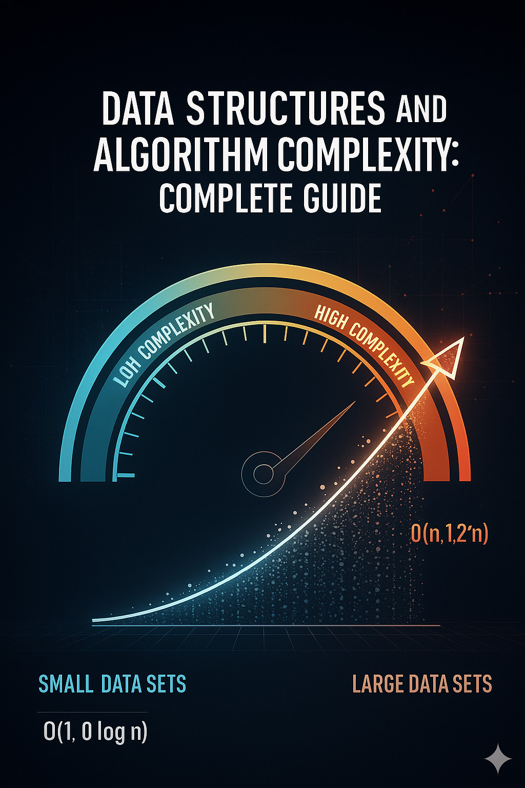
But as it scales up from a couple of hundred items to millions, how do developers ensure that their solution will still be efficient? The secret to the solution lies in the field of performance prediction, or computational complexity analysis.
| Key Takeaways: |
|---|
|
The principles of data structures, time and space complexity, and the logic that differentiates scalable systems from cunning hacks will all be covered in this guide. This is your holistic guide whether you are trying to figure out why “O(n²)” sounds like a warning sign, enhancing production software, or getting ready for coding interviews.
What is Algorithmic Complexity?
Algorithmic complexity is a mathematical expression of efficiency. It offers an answer to the question, “How does an algorithm’s running time or memory usage alter as the input size (n) increases?”
We utilize the method of asymptotic analysis, which overlooks constants and lower-order terms, and assess performance trends for a large n, to fairly compare algorithms.
Time vs Space Complexity
| Type | Definition | Example |
|---|---|---|
| Time Complexity | How running time grows with input size. | Sorting a list of 1,000 vs 1,000,000 elements. |
| Space Complexity | How memory use grows with input size. | Recursive calls create new stack frames. |
An algorithm may be memory-efficient but slow, or it may be quick but memory-hungry. Both are often balanced in real-world systems.
Understanding Asymptotic Notation
Big O, Big Θ (Theta), and Big Ω (Omega) are the most often utilized notations in algorithm analysis.
Big O Notation (Upper Bound)
The worst-case scenario, or the longest time an algorithm could take, is defined by Big O.
def find_element(arr, key):
    for item in arr:
        if item == key:
            return True
    return False
This linear search scans each element → O(n).
Big Ω (Omega) — Best Case
Ω describes the best case. For the same function, if the key is detected at the first position → Ω(1).
Big Θ (Theta) — Average Case / Tight Bound
Θ defines when upper and lower bounds are the same. If an algorithm always takes linear time regardless of input, it’s Θ(n).
Common Complexity Classes
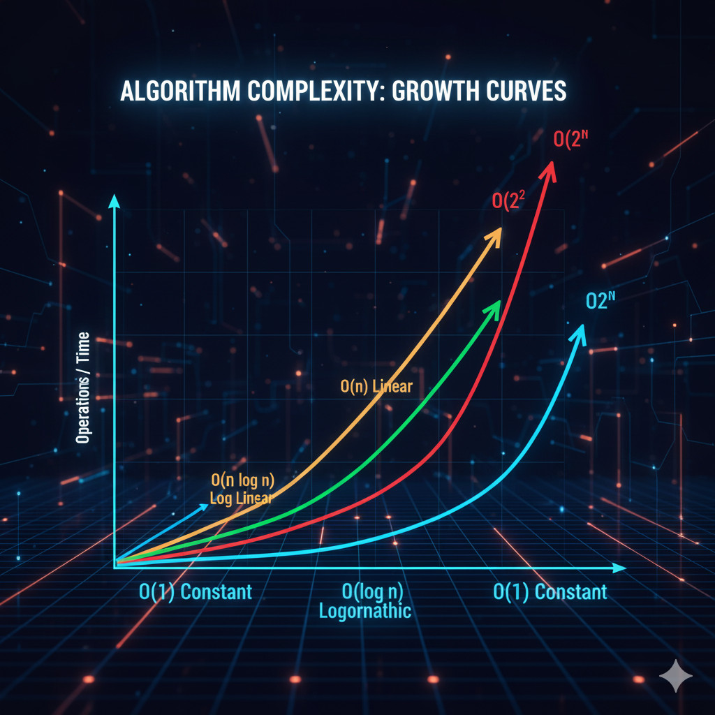
Different algorithms are segregated into general complexity classes, often viewed as growth curves.
| Complexity | Description | Example Algorithm |
|---|---|---|
| O(1) | Constant time | Accessing an array element |
| O(log n) | Logarithmic | Binary Search |
| O(n) | Linear | Linear Search |
| O(n log n) | Log-linear | Merge Sort, Heap Sort |
| O(n²) | Quadratic | Bubble Sort |
| O(2ⁿ) | Exponential | Recursive Fibonacci |
| O(n!) | Factorial | Traveling Salesman brute force |
The main objective is almost always to stay at or below O(n log n) for scalable systems.
Time Complexity in Practice
Calculate the number of times fundamental operations are performed in relation to input size to estimate time complexity.
for i in range(n):        # O(n)
    for j in range(n):    # Nested loop → O(n²)
        print(i, j)
def factorial(n):
    if n <= 1:
        return 1
    return n * factorial(n-1)
Each recursive call reduces n by 1 → O(n).
Using the Master Theorem, divide and conquer algorithms such as merge sort establish recurrence relations (e.g., T(n) = 2T(n/2) + O(n)) → O(n log n).
Space Complexity — The Forgotten Half
def sum_recursive(n):
    if n == 0:
        return 0
    return n + sum_recursive(n - 1)
Each recursive call adds a stack frame → O(n) space.
Iterative versions, by comparison, often utilize O(1) additional space.
Algorithms and Operation Complexities in Data Structures
The relevant data structure is the base of effective algorithms. Let’s review the comparison of common ones.
Arrays
| Operation | Average Time | Space | Notes |
|---|---|---|---|
| Access | O(1) | O(n) | Direct index access |
| Search | O(n) | Linear scan | |
| Insert / Delete | O(n) | Requires shifting elements |
Linked Lists
| Operation | Average Time | Space | Notes |
|---|---|---|---|
| Access | O(n) | O(n) | Sequential traversal |
| Insert at the head | O(1) | Easy to add nodes | |
| Delete | O(1) (if pointer known) | Needs a reference to the node |
stack = []
stack.append(10)  # Push O(1)
stack.pop()       # Pop O(1)
Hash Tables
| Operation | Average Time | Worst Case | Notes |
|---|---|---|---|
| Insert | O(1) | O(n) | Depends on hash collisions |
| Search | O(1) | O(n) | |
| Delete | O(1) | O(n) |
When hash functions are inaccurate, worst-case behavior degrades to linear time.
Trees
| Type | Insert | Search | Delete | Notes |
|---|---|---|---|---|
| Binary Search Tree | O(h) | O(h) | O(h) | h = tree height |
| Balanced BST (AVL/Red-Black) | O(log n) | O(log n) | O(log n) | Self-balancing |
| Heap | O(log n) | O(1) (peek) | O(log n) | Min/Max retrieval is efficient |
Graphs
| Operation | Adjacency List | Adjacency Matrix |
|---|---|---|
| Space | O(V + E) | O(V²) |
| Add Edge | O(1) | O(1) |
| Check Edge | O(V) | O(1) |
| Traversal | O(V + E) | O(V²) |
Analyzing Algorithm Complexity — Step by Step
def find_pair(arr, target):
    for i in range(len(arr)):           # O(n)
        for j in range(i + 1, len(arr)):  # O(n)
            if arr[i] + arr[j] == target:
                return True
    return False
Each nested loop → comparisons → O(n²).
def find_pair_optimized(arr, target):
    seen = set()
    for num in arr:
        if target - num in seen:
            return True
        seen.add(num)
    return False
O(n) time and O(n) space are now linear; this is an illustration of trading space for time.
Choosing the Right Data Structure
The real art lies in choosing the accurate data structure for your use case.
| Requirement | Best Choice | Reason |
|---|---|---|
| Fast lookups | HashMap | Average O(1) search |
| Sorted data | Balanced BST | O(log n) traversal |
| Constant-time insertion | Linked List | Append or prepend efficiently |
| Priority-based tasks | Heap | O(log n) extraction |
| Graph algorithms | Adjacency List | Efficient for sparse graphs |
A program that works well on a small scale may come to a complete stop when challenged with large input sizes due to poor selection.
The Trade-off: Time Complexity vs Space Complexity
An important rule is that faster algorithms tend to use more memory.
| Example | Time | Space | Comment |
|---|---|---|---|
| Recursive Fibonacci | O(2ⁿ) | O(n) | Naive recursion |
| Dynamic Programming Fibonacci | O(n) | O(n) | Stores intermediate results |
| Iterative Fibonacci | O(n) | O(1) | Best tradeoff |
Limitations of the system determine the trade-off between speed and space (e.g., servers may emphasize time while embedded systems may look at space).
Complexity Analysis in Real Life
Even though they look very abstract, complexity analyses do play out in real-world systems on a daily basis.
- O(1) hash lookups and O(log n) tree-like indices are the primary components of search engines.
- Databases utilize balanced tree structures, or B-trees, to enhance queries.
- Graph traversal and sorting are crucial for efficient machine learning pipelines.
- The exponential time complexity of blockchain encryptions and validation algorithms has necessitated further optimizations.
“Code that scales” and “code that works” are differentiated by an in-depth understanding of algorithmic complexity.
Advanced Topics in Algorithm Complexity
Amortized Analysis
- Some operations are cheap on average, but they may be costly sometimes.
- For example, dynamic array resizing has an amortized time per insertion of O(1), even though resizing is O(n).
Probabilistic and Randomized Algorithmics
- These boost the expected time complexity by using randomness.
- For example, randomized quicksort has an average-case O(n log n), worst-case O(n²).
Complexity Classes — P, NP, and Beyond
We are stepping into the segment of theoretical computer science when we discuss P, NP, and NP-complete.
- P: Issues that can be resolved in polynomial time.
- NP- Verifiable solutions in polynomial time.
- NP-complete: Issues for which there is no known polynomial-time solution.
Knowing and understanding the above allows engineers to recognize when a problem is fundamentally difficult and cannot be solved by a clever data structure.
Case Study: Sorting Algorithms and Their Complexities
| Algorithm | Best | Average | Worst | Space | Stable |
|---|---|---|---|---|---|
| Bubble Sort | O(n) | O(n²) | O(n²) | O(1) | Yes |
| Merge Sort | O(n log n) | O(n log n) | O(n log n) | O(n) | Yes |
| Quick Sort | O(n log n) | O(n log n) | O(n²) | O(log n) | No |
| Heap Sort | O(n log n) | O(n log n) | O(n log n) | O(1) | No |
While it uses more memory, merge sort guarantees performance. Although quicksort runs the risk of O(n²) on bad pivots, it is actually swifter due to cache efficiency.
Measuring Complexity Empirically
While profiling validates reality, mathematical analysis offers theory.
import timeit

setup = "from __main__ import find_pair_optimized; arr = list(range(10000))"
print(timeit.timeit("find_pair_optimized(arr, 9999)", setup=setup, number=10))
Practical engineers always verify with real data.
Best Practices for Writing Efficient Code
Writing effective code needs an engineer’s mindset, not memorization of Big O formulas.
The methods below, useful, tried, and true methods, will help you make better design choices.
Think in Terms of Growth, Not Just Output
- What would happen if my input size doubled?
- You have a scaling issue waiting to happen if the runtime quadruples or worse (O(n²)), but if it doubles, that’s fine (O(n)).
Profile Before You Optimize
- Bottleneck locations are often calculated by developers, and they are usually incorrect.
- To find out which functions really take up time, utilize profilers like Chrome DevTools for JavaScript or cProfile in Python.
- Use data, not intuition, to optimize.
Know Your Data Structures by Heart
Every data structure is a machine that makes trade-offs easier:
- Need swift lookups? → Hash Map.
- Need sorted data? → Balanced Tree.
- Need to often add/remove from both ends? → Deque.
An O(1) operation can fast become an O(n) operation with a wrong decision.
Cache Repeated Work
Recomputing values is a silent performance killer.
from functools import lru_cache

@lru_cache(maxsize=None)
def fib(n):
    if n <= 1: return n
    return fib(n-1) + fib(n-2)
Use Efficient Libraries
- You don’t always have to start from scratch when working with real-world systems.
- Leverage libraries that have been expertly optimized and validated for efficiency, like C++ STL containers or NumPy (vectorized operations).
Measure Constant Factors
- Despite their elegant appearance, recursive functions can lead to memory usage issues or stack overflows.
- Loops are often more space-efficient, but tail recursion optimization is useful in some languages.
Measure Constant Factors
- Constants are important, but Big O hides them.
- An O(n log n) algorithm with lightweight operations may still outperform an O(n) algorithm with a lot of computation inside the loop.
Use Space to Save Time (and Vice Versa)
- If you can afford some additional memory, caching or indexing can reduce the runtime dramatically. If you are working with an embedded system or mobile app, do the opposite: prioritize space efficiency.
Practice Reading Other People’s Code
- Minor design decisions such as loop placement, data structure nesting, and memory reuse often conceal efficiency.
- Real-world optimization patterns can be identified by reading open-source code, such as React internals or CPython.
Common Mistakes in Complexity Analysis
When n is small, constants are overlooked.
- Prematurely over-engineering for performance.
- Not knowing the difference between the average and worst cases.
- Ignoring the space constraints.
- Ignoring hidden complexity (hashing, string operations).
- Algorithms don’t work in a vacuum; always contextualize your analysis.
Complexity in Modern Contexts
Contemporary systems, such as cloud and artificial intelligence, take complexity thinking even further:
- Distributed systems: Network latency and data sharding determine complexity.
- Streaming algorithms: To process infinite input streams, use O(1) or O(log n) space.
- Parallel computing: While synchronization can increase overhead, task division can reduce effective time.
Even when hardware scales horizontally, understanding algorithmic efficiency is still vital.
Mastering Data Structures and Complexity
At its heart, Data Structures and Algorithm Complexity is about understanding how your code grows. These imperceptible mathematical patterns impact every application, from a small script to a large distributed system.
Big O table memorization is not a prerequisite for mastering complexity. It means:
- Knowing which data structure can convert an O(n²) search into an O(1) search.
- Identifying when a nested loop is a ticking time bomb.
- Knowing when it makes sense to use more memory in order to save time, or vice versa.
- Building systems that, even when n grows enormous, maintain their elegance under pressure.
Developers who understand algorithmic efficiency build better experiences rather than just better code in a world where data is everywhere.
Because ultimately, every millisecond saved is useful to people, it is the difference between waiting and moving forward.
Additional Resources
- Why Learning Data Structures and Algorithms (DSA) is Essential for Developers
- What is Code Optimization?
- Searching vs Sorting Algorithms: Key Differences, Types & Applications in DSA
|
|