What is the Square Root (Sqrt) Decomposition Algorithm?
Every programmer eventually asks, “Is it possible to make my queries without rebuilding everything every single time?” when working with massive datasets and often running array queries.
The Square Root Decomposition Algorithm, or sqrt algorithm, comes into play at this point. You can respond to questions in sublinear time with this elegant and surprisingly simpler method that cuts larger problems into smaller, balanced chunks. One of the simplest methods for designing algorithms, it acts as a link between innovative data structures like segment trees and Fenwick trees and brute-force methods.
| Key Takeaways: |
|---|
|
Let us take a closer look and learn the sqrt algorithm from the ground up.
The Core Idea Behind Square Root Decomposition
Square Root Decomposition’s basic idea is simple but effective.
Precompute partial results for each block of the array after dividing it into equal-sized blocks (roughly the square root of the total number of elements).
The mathematical concept that each block will entail approximately √Nelements when Nelements are divided into √N blocks is the source of this idea. A sweet spot between query efficiency and precomputation cost is offered by this balance.
In essence:
- You preprocess blocks in O(N) time.
- You answer each query in O(√N) time.
- You can handle point updates in O(1) time.
So, the Square Root Algorithm effectively decreases the amount of work needed for each query while maintaining a low level of preprocessing.
Why Is It Called the “Square Root” Algorithm?
The Square Root Decomposition Algorithm’s name, “square root”, isn’t a coincidence; it directly refers to the block size selection.
- You divide it into blocks of size B=√N.
- There are √Nblocks in total.
- Each block holds √Nelements.
The overall time complexity becomes proportional to √N since the majority of the computations (queries and updates) include traversing or referencing about √N elements or blocks. That’s why it’s called the Square Root Algorithm, or just the Sqrt Algorithm.
The Problem It Solves
- Range Query: Determine a subarray’s sum (or minimum/maximum) [L,R].
- Point Update: Make one change to arr[i] = val.
For large datasets or frequent queries, the O(N) time needed for the brute-force solution to each range query is impractical.
This could be resolved with a segment tree or binary indexed tree, but their implementation is more intricate.
A compromise is provided by square root decomposition, which is easier to use than tree-based techniques and faster than brute force.
The Structure of the Sqrt Algorithm
Use these procedures to put the Square Root Decomposition Algorithm into practice:
Step 1: Divide the array into blocks.
- Assume that N = 16.
- The block size is √16=4.
- The array is divided into four blocks, each of which has four elements.
Block Elements
| Block | Elements |
|---|---|
| 0 | arr[0] – arr[3] |
| 1 | arr[4] – arr[7] |
| 2 | arr[8] – arr[11] |
| 3 | arr[12] – arr[15] |
Step 2: Precompute Block Information
We precompute the required information (like sum, min, or max) for each block.
Example for sum:
blockSum[0] = arr[0] + arr[1] + arr[2] + arr[3]

blockSum[1] = arr[4] + arr[5] + arr[6] + arr[7]

...
This preprocessing is O(N).
Step 3: Answer Questions Effectively
Regarding a range query [L, R]:
Do a direct calculation if L and R are in the same block.
- To the end of L’s block, add the partial sum from L.
- Use precomputed sims to add all complete blocks in between.
- Add to R the partial sum from the beginning of R’s block.
Now, O(√N) time is needed for each query.
Step 4: Respond to Updates
You just need to update the block summary for each element that has been altered.
The time needed for this is O(1).
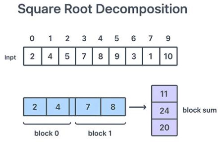
Example: Range Sum Query with Square Root Decomposition
Let us use a simple sum query issue to demonstrate the sqrt algorithm.
Given:
arr = [2, 4, 5, 7, 8, 9, 3, 1, 6, 10]

N = 10 ⇒ block size = √10 ≈ 3
- Block 0:
[2, 4, 5]→ sum = 11 - Block 1:
[7, 8, 9]→ sum = 24 - Block 2:
[3, 1, 6]→ sum = 10 - Block 3:
[10]→ sum = 10
Query: Find the sum from index 2 to 8.
- Partial (end of block 0): arr[2] = 5
- Full blocks (1): sum = 24
- Partial (start of block 2): arr[6] + arr[7] + arr[8] = 3 + 1 + 6 = 10 Total = 5 + 24 + 10 = 39
Complexity:
Pseudocode for Square Root Algorithm
import math

def build_sqrt_decomposition(arr):
    n = len(arr)
    block_size = int(math.sqrt(n))
    block_sum = [0] * ((n + block_size - 1) // block_size)
    for i in range(n):
        block_sum[i // block_size] += arr[i]
    return block_sum, block_size

def query(arr, block_sum, L, R, block_size):
    sum_val = 0
    while L <= R and L % block_size != 0:
        sum_val += arr[L]
        L += 1
    while L + block_size - 1 <= R:
        sum_val += block_sum[L // block_size]
        L += block_size
    while L <= R:
        sum_val += arr[L]
        L += 1
    return sum_val

def update(arr, block_sum, idx, val, block_size):
    block_idx = idx // block_size
    block_sum[block_idx] += val - arr[idx]
    arr[idx] = val
- Preprocessing: O(N)
- Query: O(√N)
- Update: O(1)
Applications of the Square Root Decomposition Algorithm
Surprisingly adaptable, the square root algorithm can be used to resolve a wide range of computational issues:
Range Sum / Range Min / Range Max Queries
- The simplest use is to calculate aggregate properties over a subarray quickly.
Range Frequency Queries
- Effectively compute instances of an element within a range.
Prefix Operations
- For swift lookups, use sqrt decomposition to precompute prefix sums or prefix minimums.
2D Arrays
- For 2D queries, square root decomposition can be extended to matrices, splitting them into √N x √N subgrids.
Competitive Programming
- It is frequently used when full segment trees are unnecessary for problems involving static queries.
The Square Root Decomposition is the preferred method for moderate constraints due to its simplicity and clarity, even though it is somewhat slower asymptotically.
Mo’s Algorithm: An Extension of Square Root Decomposition
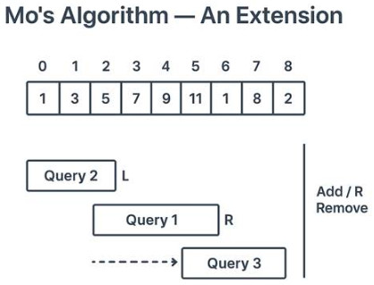
Let us now take a look at Mo’s Algorithm, a well-known extension of the sqrt algorithm,
What is Mo’s Algorithm?
Mo’s Algorithm is a Square Root Decomposition-based offline query optimization method.
- When the array is static (does not change between queries).
- You have a number of range queries with computation reuse capabilities.
- Mo’s algorithm cleverly rearranges the queries to reduce query window movements rather than recomputing answers from scratch.
How does Mo’s Algorithm Work?
As with the sqrt decomposition, divide the array into blocks of size √N.
Sort queries as per:
- Their right index (either descending or ascending, depending on the situation).
- Maintain a sliding window while processing queries one after the other [L, R].
- To match the range of each query, move L and R incrementally, adding or deleting elements as you go.
This reduces the cost of switching between queries to O(√N), and the time needed for each addition or removal is constant.
Complexity
If there a Q questions:
Total complexity: O((N+Q)*√N)
- Number of distinct elements in a range
- Sum of a subarray
- Range XOR queries
- Frequency-related computations
Mo’s algorithm is described as a “next level” sqrt algorithm that efficiently reuses intermediate results between queries.
Advantages of Square Root Decomposition
The Square Decomposition Algorithm is a prominent tool in algorithm design, competitive programming, and even some real-world applications because of its many theoretical and practical advantages. Let us take a closer look at these advantages:
Simplicity and Ease of Implementation
The sqrt algorithm’s ease of writing and reasoning is one of its greatest benefits. Recursive tree structures and complex update mechanisms are not needed.
An array, a few loops, and a fundamental knowledge of how to split data into blocks of size √N.
It offers a clear introduction to the idea of partial precomputation, which is the basis of many innovative algorithms, for students and freshers learning data structures.
Balanced Time Complexity
Between brute-force and logarithmic data structures, the sqrt algorithm finds a sweet spot.
For moderately sized datasets, where segment trees or binary indexed trees might be overkill, this balanced complexity is ideal.
Great for Static or Semi-Static Data
The Square Root Decomposition Algorithm works well when your dataset doesn’t change much, such as when updates are scarce or only occur at certain times. It allows low overhead and fast query processing.
A segment tree, in comparison, may take longer to maintain equilibrium or recompute internal nodes for sporadic updates.
Space Efficiency
Sqrt decomposition only needs a small auxiliary array to store block summaries, as compared to a segment tree, which may take up almost twice as much space as the original data.
It is memory-friendly for embedded systems or competitive programming environments because it usually uses less than 1.5x the memory footprint of the original dataset.
Flexibility in Operations
- Minimum or maximum over a range
- Frequency counting
- XOR or GCD queries
- Custom associative operations
Because of its versatility, sqrt decomposition is a viable option for issues related to specialized query logic.
Ideal for Teaching and Debugging
The algorithm is perfect for teaching the shift from O(N) methods to optimized O(√N) techniques.
Debugging is also made simple by its deterministic and linear block structure, which allows for independent inspection of each block.
Foundation for Advanced Algorithms
Lastly, the Square Root Algorithm offers the conceptual foundation for more intricate methods such as DSU on Trees, Mo’s Algorithm, and sqrt decomposition with lazy propagation. Mastering proficiency in it lays the groundwork for later understanding and design of an increasingly complex range query optimization.
Limitations of the Sqrt Algorithm
- Slower for Large N: Compared to O(log N) structures like segment trees or Fenwick trees, queries take O(√N), which is slower. This difference can be important for very large arrays.
- Limited Range Updates: While point updates are quick, unless more complex “lazy” variants are used, updating an entire subarray often takes O(N).
- Block Size Sensitivity: The choice of block size determines optimal performance; a bad choice may lead to uneven computation.
- Not Ideal for Dynamic Data: It is less appropriate for extremely dynamic arrays because regular insertions, deletions, or resizing require rebuilding blocks.
- Complex for Non-Associative Operations: Simple operations, such as the median or mode, are hard to execute efficiently.
- Memory Overhead in Higher Dimensions: Because 2D and 3D need more block summaries, memory usage increases noticeably.
Choosing Between Sqrt Decomposition and Mo’s Algorithm
| Criterion | Square Root Decomposition | Mo’s Algorithm |
|---|---|---|
| Query Type | Online (processed as they come) | Offline (all known beforehand) |
| Updates | Supported | Not supported |
| Complexity | O(√N) per query | O((N + Q)√N) total |
| When to Use | Moderate N, online operations | Many static queries, reuse possible |
Advanced Variants and Optimizations
- Lazy propagation in Sqrt Decomposition: Store lazy values at the block level to manage range updates.
- Sqrt Decomposition on Graphs or Trees: Can be adapted using Euler Tour + block partitioning.
- 2D Sqrt Decomposition: Divide both dimensions into √N x √N blocks for effective range queries in matrices.
- Hybrid Models: Integrate Sqrt Decomposition with Segment Tree or BIT for specific applications.
Real-World Examples
- Data Analytics: Fast aggregation of time series data over windows.
- Game Development: Player statistics are updated in segments in an efficient manner.
- Finance: Executing searches on past stock ranges.
- Competitive Programming: Often used in range problem competitions.
Conclusion
Complex data structures are not always necessary for efficient optimization, as explained by the Square Root (Sqrt) Decomposition Algorithm. It achieves efficient querying with little overhead by utilizing basic mathematical intuition, which involves splitting data into √N blocks.
The sqrt algorithm is a good example of balanced design in today’s world of massive data, where simplicity and performance often need to coexist.
The square root method is more than just a trick; it is a basic concept in algorithmic problem solving. Mo’s Algorithm expands on this idea for innovative offline query handling when you need to push it further.
|
|