Greedy Algorithm in Data Structures: A Complete Guide
Algorithms are at the heart of data structures and computer science. An algorithm contains the complete and precise logical procedure for solving problems. There are different paradigms in algorithm design, such as dynamic programming, backtracking, and divide-and-conquer. Of these techniques, the greedy algorithm is notable for its simplicity and (in some cases) optimality.
| Key Takeaways: |
|---|
|
This guide on greedy algorithms will delve into what greedy algorithms are, how they work, where they are used, and some common programming problems that use the algorithm to reach a solution.
What is a Greedy Algorithm?
A greedy algorithm is a problem-solving algorithmic strategy that builds a solution step by step, always choosing the next step that offers the most immediate benefit or the “best” local choice, without considering the future.

In other words, at each step, the greedy algorithm assumes that the current choice will lead to a globally optimal solution. Once a selection is made, it is never reconsidered.
It focuses on taking the most immediate, obvious solution that will work best right now. Thus, even if a better path becomes available later, it does not revisit or revise earlier decisions.
In greedy algorithms, you focus on the individual sub-models of a bigger problem and try to solve them independently.
Key Characteristics of Greedy Algorithms
- Greedy algorithms make locally optimal choices by making decisions based on the current best option.
- It does not look ahead or revisit previous steps. Once a choice is made, it cannot be changed later. This makes greedy algorithms fast, but they can sometimes be unable to correct earlier mistakes, especially in complex scenarios.
- While greedy algorithms are practical for many problems, they do not always guarantee a globally optimal solution. In some cases, like the Traveling Salesman Problem, they can even produce the worst-case output.
- Greedy algorithms are generally faster and use less memory compared to approaches like dynamic programming, which consider all possible combinations and require storing intermediate results.
- Greedy algorithms are easy to understand and implement; however, proving their correctness mathematically can be complex.
- Greedy algorithms can provide a near-optimal or approximate solution that is good enough for practical use, especially in problems where finding an exact solution is computationally infeasible.
History of Greedy Algorithm
- Greedy algorithms were developed for various graph traversal algorithms in the 1950s.
- In the same decade, Prim and Kruskal developed optimization strategies based on minimizing path costs along weighted routes.
- Edsger Dijkstra proposed the concept of greedy algorithms to generate minimum spanning trees. He wanted to shorten the routes in Amsterdam.
- In the ’70s, American researchers Cormen, Rivest, and Stein put forward a proposal for recursive substructuring of greedy solutions in their book “ Introduction to Algorithms”.
- The greedy search paradigm was registered as a different type of optimization strategy in the NIST records in 2005.
- To date, protocols that run the web, such as the open shortest path first (OSPF) and many other network packet switching protocols, use the greedy strategy to minimize time spent on a network.
Real-Life Analogy for Greedy Algorithms
Imagine you are collecting coins/notes to reach a certain amount in a stipulated time. You are applying a greedy approach if you always pick the highest denomination available first (for example, the Rs 10 note before the Rs 5). It may not always be the optimal solution, but in a standard currency system, it works fine.
As another example, imagine you are hungry and want to eat something. You walk into a cafe with different food options. You have only a few coins with you, and you want to get the most food for your money to satisfy your hunger.
A greedy approach would be to examine all the food, select the one that yields the most value for your coins, purchase it, and then repeat with the remaining coins. You’re not planning for what you might want later, just grabbing the best deal you see right now.
In some cases, the greedy approach is practical and yields the best possible results. In some instances, it may not produce the best overall outcomes, but it is a quick and easy way to resolve the problem.
Key Concepts of the Greedy Algorithm
The following two fundamental properties aid in designing a greedy algorithm:
1. Greedy Choice Property
According to the greedy choice property, an optimal solution can be achieved by making a sequence of locally optimal choices, or greedy choices, in each step.
The choice made at each step is independent of future choices and won’t be reversed later once the decision is made. This property means that the choice made at each step is the best one available at that moment.
For example, in the Fractional Knapsack Problem, selecting the item with the highest value-to-weight ratio at each step leads to the global optimum.
2. Optimal Substructure
A problem has optimal substructure if an optimal solution to the problem contains optimal solutions to its subproblems.
According to the optimal substructure property, a problem can be broken down into smaller subproblems, and these subproblems can be solved optimally to reach the optimal solution of the overall problem. Thus, an optimal solution for a problem consists of optimal solutions for its subproblems.
In shortest path problems such as Dijkstra’s algorithm, the shortest path from a source to a destination includes the shortest path from the source to intermediate nodes.
How a Greedy Algorithm Works?
Greedy algorithms solve problems by following a simple, step-by-step approach as follows:
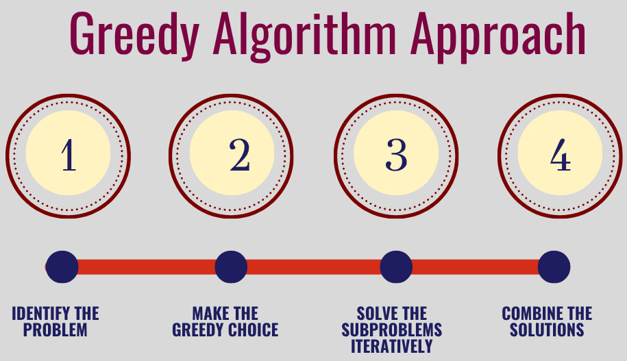
- Identify the Problem: A greedy approach begins with understanding the problem and determining whether it can be solved using a greedy approach. It is assessed to see if it can be broken down into a series of decisions where a locally optimal choice at each step contributes to a potentially globally optimal solution.
- Make the Greedy Choice: At each step of the problem, a choice is made that seems optimal at the moment. The choice is based on the greedy choice property, selecting the option that offers the most immediate benefit. This step might involve choosing the largest, smallest, shortest, or most profitable option available at that moment.
- Solve the Subproblems Iteratively: Once the greedy choice is made, the problem is then reduced to smaller subproblems. The greedy choice is applied repeatedly, building the solution incrementally until the problem is solved or no further greedy decisions can be made.
- Combine the Solutions: Once the entire problem is solved by iteratively solving the subproblems, the solution to the overall problem is simply the combination of all the greedy choices made at each step.
Greedy Algorithm vs Dynamic Programming
Greedy and dynamic programming approaches rely on the principle of optimal substructure. However, they differ fundamentally in their approach. Here are the key differences between the greedy algorithm and dynamic programming:
| Feature | Greedy Algorithm | Dynamic Programming |
|---|---|---|
| Decision Making | Makes local optimal choices at each step | Makes global optimum choices through subproblem solution and explores all possibilities |
| Optimality Guarantee | Solution is not always guaranteed | Guaranteed solution for suitable problems |
| Backtracking | None (irrevocable decisions) | Uses previously computed results |
| Problem Structure | Greedy choice property | Optimal substructure & overlapping subproblems |
| Complexity | Generally, lower time complexity | Can have higher time and space complexity |
| Approach | Follows a top-down approach in concept (making a choice and solving the rest) | Follows a bottom-up approach (solving subproblems first) or top-down with memorization |
| Efficiency | Fast and simple | Slower but more reliable |
| Examples | Minimum Spanning Tree, Shortest Path algorithms | Fibonacci sequence, Longest Common Subsequence |
In essence, greedy algorithms are fast but not always accurate, or they are “short-term thinkers”. Dynamic programming algorithms, on the other hand, are “strategic thinkers”, slow but guaranteed output.
Greedy Algorithms: Real-Life Applications and Examples
Greedy algorithms find application in various computational problems where a locally optimal choice at each step leads to a globally optimal solution. Here are some key applications:
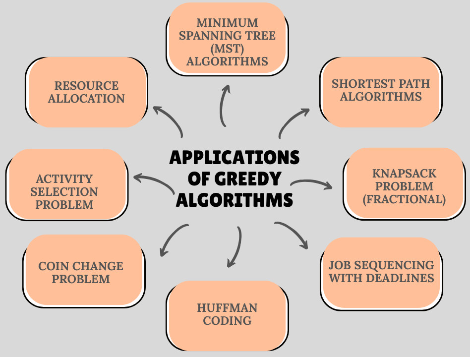
1. Minimum Spanning Tree (MST) Algorithms
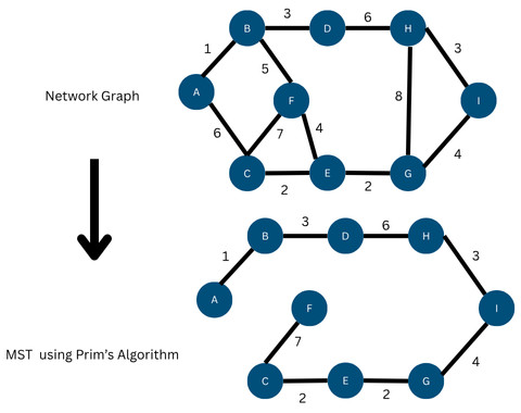
- Prim’s Algorithm: This algorithm builds an MST by iteratively adding the cheapest edge connecting a vertex in the growing tree to a vertex outside the tree. The steps are:
- Start Vertex: Begin with an arbitrary starting vertex and add it to the MST.
- Grow MST: Select the minimum-weight edge that connects the vertex already in MST to a vertex not yet in MST. Add a new vertex to the MST.
- Termination: Repeat the process of adding vertices to the MST until all vertices are exhausted.
A priority queue is often used to find the minimum-weight edge in each step efficiently.
Example: The following figure shows an MST obtained using Prim’s algorithm:
- Kruskal’s Algorithm: This algorithm constructs an MST by adding edges in increasing order of weight, as long as they don’t form a cycle. Kruskal’s algorithm follows these steps:
- Sort Edges: All edges in the graph are sorted in increasing order of their weights.
- Initialize Forest: Each vertex is initially considered as a separate component (a forest of single-node trees).
- Add Edges: Iterate through the sorted edges. For each edge, if it connects two vertices that are currently in different components (i.e., adding the edge does not form a cycle), add the edge to the MST and merge the two elements.
- Termination: The algorithm terminates when the MST contains n-1 edges, where n is the number of vertices in the graph.
Example: The following image shows an example of Kruskal’s algorithm with an input graph and MST:
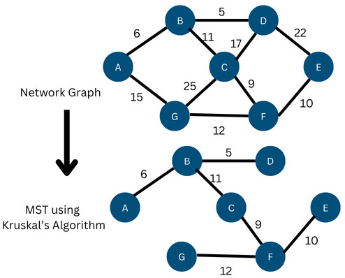
Here, initially, the edges are sorted in ascending order as per their weights. Next, as each vertex is visited, the edge with the least cost is added to the MST, ensuring there is no cycle.
2. Shortest Path Algorithms
- Dijkstra’s Algorithm: This algorithm works by iteratively finding the closest unvisited vertex, updating the distances to its neighbors (a process known as “relaxation”), and marking it as visited until all vertices have been exhausted. The steps followed in the algorithm are:
- Initialization:
- Set the distance to the source vertex to zero and all other distances to infinity.
- Create a set to keep track of visited vertices.
- Iteration:
- While there are unvisited vertices:
- Select the unvisited vertex u with the smallest current distance.
- Mark u as visited.
- For each neighbor v of u:
- Relax the edge: If the distance to u plus the edge weight from u to v is less than the current distance to v, update the distance to v and record u as the previous vertex on the shortest path to v.
- While there are unvisited vertices:
- Result: The final distances and recorded previous vertices allow you to reconstruct the shortest path from the source to any other vertex.
- Initialization:
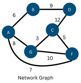
Example: The following figure shows the graph for which the shortest path is to be found.
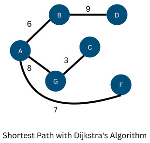
As per Dijkstra’s algorithm, the output is the following figure:
3. Knapsack Problem (Fractional)
This is an optimization problem where the goal is to select items with associated weights and values to maximize the total value in a knapsack of limited capacity. The key feature of this problem is the ability to divide items into fractions.
It’s solved using a greedy approach by sorting items by their value-to-weight ratio in descending order and then adding them to the knapsack, taking whole items until the next item would exceed the capacity. At that point, only a fraction of the last item is taken to fill the knapsack.
- Calculate Value-to-Weight Ratio: For each item, compute its value-to-weight ratio (value/weight).
- Sort Items: Sort all items in descending order of their calculated value-to-weight ratios.
- Fill the Knapsack:
- Start with the item having the highest value-to-weight ratio.
- If the item’s full weight can fit in the remaining capacity, add it entirely and update the knapsack’s remaining capacity and total value.
- If the item’s full weight exceeds the remaining capacity, add only the fraction of the item that will fill the knapsack to its maximum capacity.
- Continue this process until the knapsack’s capacity is zero.
Example:
Consider a knapsack with a capacity of W = 50. There are three items available, each with a specific value and weight. Using the algorithm steps listed above, we first calculate the value-to-weight ratio for each item. The following table shows this data:
| Items | Value | Weight | Value-to-Weight Ratio |
|---|---|---|---|
| Item 1 | 60 | 10 | 60 / 10 = 6 |
| Item 2 | 100 | 20 | 100 / 20 = 5 |
| Item 3 | 120 | 30 | 120 / 30 = 4 |
- Item 1 (Ratio = 6)
- Item 2 (Ratio = 5)
- Item 3 (Ratio = 4)
- Item 1: The knapsack has a capacity of 50. Item 1 weighs 10. Since 10 <= 50, take the entire Item 1.
Current Value = 60; Remaining Capacity = 50 – 10 = 40
- Item 2: The remaining capacity is 40. Item 2 weighs 20. Since 20 <= 40, take the entire Item 2.
Current Value = 60 + 100 = 160; Remaining Capacity = 40 – 20 = 20
- Item 3: The remaining capacity is 20. Item 3 weighs 30. Since 30 > 20, a fraction of Item 3 must be taken.
Fraction of Item 3 to take = Remaining Capacity / Item 3 Weight = 20 / 30 = 2/3Value contributed by the fraction = (2/3) * 120 = 80Current Value = 160 + 80 = 240; Remaining Capacity = 20 – ((2/3) * 30) = 0
Conclusion: The maximum value that can be obtained in the knapsack is 240, achieved by taking the entire Item 1, the whole Item 2, and 2/3 of Item 3.
4. Job Sequencing with Deadlines
- Sort Jobs: Sort the given jobs in descending order of their profit.
- Determine Max Deadline: Find the maximum deadline among all jobs to determine the total number of available time slots.
- Initialize Time Slots: Create an array or data structure (e.g., a hash array) to represent the time slots, all initially marked as empty.
- Iterate and Schedule:
- Iterate through the sorted jobs.
- For the current job, iterate backward from its deadline to day zero.
- Find the latest available empty time slot within its deadline.
- If an empty slot is found, assign the job to that slot, record the job’s ID, and add its profit to the total profit.
- Result: The selected jobs in the filled slots constitute the optimal schedule that maximizes profit.
Example:
Given n jobs with deadlines and profits, schedule jobs to maximize profit where each job takes one unit of time.
- Sort jobs in descending order of profit.
- Assign each job to the latest available slot before its deadline.
- Skip if no slot is available.
5. Huffman Coding
This is a lossless data compression technique that employs a greedy approach to construct an optimal prefix-free binary tree, assigning variable-length codes to input characters based on their frequencies. The core principle of this problem is to use shorter codes for frequently occurring characters and longer codes for less frequent ones, thereby reducing the overall size of the data.
- Frequency Calculation: The frequency of each character in the input data is determined.
- Huffman Tree Construction:
- Create a leaf node for each character, representing its frequency.
- Repeatedly combine the two nodes with the lowest frequencies into a new parent node, whose frequency is the sum of its children’s frequencies.
- Continue this process until only one node (the root of the Huffman tree) remains.
- Code Assignment: Traverse the Huffman tree from the root to each leaf node. Assign a ‘0’ to left branches and a ‘1’ to right branches. The path from the root to a character’s leaf node forms its unique Huffman code.
- Encoding: Replace each character in the original data with its corresponding Huffman code.
- Decoding: To decode, traverse the Huffman tree using the encoded bitstream. When a leaf node is reached, the corresponding character is identified.
6. Coin Change Problem
In many standard currency systems, a greedy algorithm can be used to provide change using the minimum number of coins by repeatedly selecting the largest denomination coin less than or equal to the remaining amount.
7. Activity Selection Problem
In this problem, the maximum number of non-overlapping activities is selected from a given set, where each activity has a start and finish time, by prioritizing activities that finish earliest.
8. Resource Allocation
Greedy strategies can be used in various resource allocation scenarios, such as prioritizing tasks or data syncing in mobile applications based on urgency or importance.
Advantages of Greedy Algorithms
- Simplicity: Greedy algorithms are easy to understand and implement. They are straightforward and often require minimal code.
- Efficiency: They are typically faster due to their single-pass decision-making process and have low time complexity, providing quick solutions for specific problems.
- Fewer Resources: These algorithms use less memory since it doesn’t require recursion or table storage.
- Optimal for Many Problems: Greedy algorithms work perfectly in cases with the greedy choice property (e.g., MST, Huffman).
- Reduced Memory Usage: Their efficient nature often translates to low memory requirements and efficient use of memory resources.
- Building Blocks for Complex Algorithms: Greedy strategies can be incorporated into more sophisticated algorithms to tackle more challenging problems.
Disadvantages of Greedy Algorithms
- No Guarantee of Global Optimum: A greedy algorithm focuses on the best choice at the current moment and may result in suboptimal solutions.
- Problem-Specific: Greedy algorithms are only applicable to specific problems that exhibit the greedy choice property and optimal substructure. They may not work for all issues.
- Hard to Design Proofs: It is hard to rigorously prove that a greedy algorithm will always produce a correct or optimal solution for a specific problem.
- Lack of Flexibility: Greedy algorithms are rigid, as once a choice is made, it cannot be changed. Modifying a greedy algorithm to handle different constraints or problem variations can be challenging due to its fixed approach.
- Sensitivity to Input Order: The order in which input data is presented can significantly affect the outcome of a greedy algorithm.
- No Backtracking: The choice once made cannot be reversed or backtracked. As a result, the algorithms may be trapped in a suboptimal state if an early “greedy” choice was incorrect.
When to Use Greedy Algorithms
- The problem exhibits both greedy choice and optimal substructure properties.
- You need fast approximations for large-scale problems.
- Local decisions are both independent and cumulative in their approach toward a goal.
- Minimum Spanning Tree (Kruskal’s, Prim’s)
- Huffman Encoding
- Fractional Knapsack
- Job Scheduling
- Interval Problems
Conclusion
The greedy algorithm approach is a cornerstone of data structures and algorithm design. It is a powerful paradigm in solving optimization problems where local decisions lead to global optimal solutions. Greedy algorithms are fast and simple but have limited applicability.
Whether you’re designing efficient network routing, compressing data, or optimizing tasks, greedy algorithms offer elegant, straightforward, practical, and computationally efficient solutions. When used wisely, they transform complex problems into streamlined, solvable ones, proving that sometimes, being greedy can be beneficial.
|
|