Graphs: Difference Between BFS and DFS
The invisible wiring of our digital world is made up of graphs, which subtly fuel the programs and tools we utilize on a daily basis. You are actually viewing a graph in action, whether you are utilizing Google Maps to navigate through city streets, binge-watching a Netflix series that was “recommended for you,” or following a rumor that spreads on social media.
Relationships between cities, users, or even ideas are modeled by graphs, and machines understand and navigate these relationships using algorithms such as BFS (Breadth-First Search) and DFS (Depth-First Search).
Consider yourself in a massive escape room with multiple doors that connect to one another. Do you select one path and follow it as far as you can before turning around (like DFS), or do you first examine every room nearby before moving deeper (like BFS)?
That’s the heart of this discussion: two different mindsets for exploring complexity.
Both DFS and BFS are strategic approaches to problem-solving; one highlights depth, while the other highlights breadth. They are more than just theoretical tools. Knowing the difference between BFS and DFS can help in your reasoning when working with algorithms, as well as real-world issues that mimic pattern recognition, exploration, and decision-making.
| Key Takeaways: |
|---|
|
By the end of this blog, you will not only understand what BFS and DFS are, but you will intuitively feel why one makes sense in certain situations while the other shines elsewhere.

What is BFS (Breadth-First Search)
A traversal algorithm called Breadth-First Search (BFS) analyzes every vertex in a graph level by level.
Before going on to the next level of neighbors, it visits each of the nodes that are adjacent to the source node. The algorithm is certain to investigate nodes in order of their distance (measured in terms of edges) from the starting point due to this “layer-by-layer” method.
How BFS works
- Begin by marking the source node as visited.
- Add it to a line.
- While the queue is not empty:
- Dequeue the front node.
- Visit all its unvisited neighbors.
- Mark each neighbor as visited and enqueue it.
- Keep going until you have visited every vertex that can be reached.
This structured method guarantees that every node is visited according to how far away it is from the beginning.
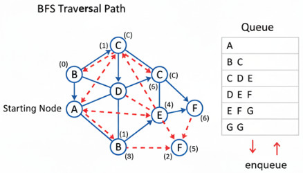
Example Diagram (BFS)
Let us consider the following simple graph:
     A

    / \

   B   C

   | \   \

   D  E   F
The adjacency list looks like this:
A: B, C

B: A, D, E

C: A, F

D: B

E: B

F: C
BFS traversal starting from A:
- Start with A → mark visited.
Queue = [A] - Dequeue A → visit its neighbors (B, C).
Queue = [B, C], visited = {A, B, C} - Dequeue B → neighbors D, E (A already visited).
Queue = [C, D, E], visited = {A, B, C, D, E} - Dequeue C → neighbor F (A visited).
Queue = [D, E, F], visited = {A, B, C, D, E, F} - Dequeue D, then E, then F — all neighbors already visited.
The queue becomes empty.
Traversal Order: A → B → C → D → E → F
This is the breadth-first order, level by level.
BFS Pseudocode
def bfs(graph, start):
    visited = set()
    queue = [start]
    visited.add(start)

    while queue:
        node = queue.pop(0)
        print(node, end=" ")

        for neighbor in graph[node]:
            if neighbor not in visited:
                visited.add(neighbor)
                queue.append(neighbor)
BFS Characteristics
- Traversal type: Level-order (breadth first)
- Data structure: Queue (FIFO)
- Completeness: Complete for finite graphs
- Shortest path: Guaranteed in unweighted graphs
- Time complexity: O(V + E)
- Space complexity: O(V) in the worst case (for the queue)
When to use BFS
- When an unweighted graph’s shortest path is needed.
- When the start node is close to the solution.
- For layered search or level-order traversal.
- When exploring social connection, unweighted paths, or grid problems (like figuring out how many steps to take in a maze).
What is DFS (Depth-First Search)
A traversal algorithm called Depth-First Search (DFS) goes as far down a branch as it can before turning around.
DFS uses a stack (Last In, First Out) in place of a queue; this is regularly done implicitly through recursion.
How DFS works
- Start at the source node.
- Mark it as visited.
- Before going on to the next neighbor, recursively visit each one that hasn’t been seen.
- Backtrack when there are no more unvisited neighbors.
- Keep going until you have visited every reachable node.
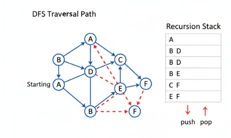
Example Diagram (DFS)
Using the same graph:
     A

    / \

   B   C

   | \   \

   D  E   F
DFS traversal starting from A:
- Start at A → visit, go to B.
- From B → go to D → backtrack to B → go to E → backtrack.
- From A → go to C → then to F.
Traversal Order: A → B → D → E → C → F
DFS Pseudocode (Recursive)
def dfs(graph, node, visited):
    if node not in visited:
        print(node, end=" ")
        visited.add(node)
        for neighbor in graph[node]:
            dfs(graph, neighbor, visited)
DFS using Stack (Iterative Version)
def dfs_iterative(graph, start):
    visited = set()
    stack = [start]

    while stack:
        node = stack.pop()
        if node not in visited:
            print(node, end=" ")
            visited.add(node)
            for neighbor in reversed(graph[node]):
                stack.append(neighbor)
DFS Characteristics
- Traversal type: Depth-first
- Data structure: Stack/recursion
- Completeness: May not be complete for infinite graphs
- Shortest path: Not guaranteed
- Time complexity: O(V + E)
- Space complexity: O(V) (for recursion stack)
When to use DFS
- When you wish to explore every node.
- When memory is scarce, BFS’s frontier may blow up.
- When working through puzzles, mazes, or backtracking.
- For connected components, SCC (Strongly Connected Components), cycle detection, and topological sorting.
- When the solution is located far down the search tree.
BFS and DFS Example – Side by Side
Let’s summarize both traversals with a single visualization.
Graph:
     A

    / \

   B   C

   | \   \

   D  E   F
BFS (Level by Level)
A → B → C → D → E → F
DFS (Depth by Depth)
A → B → D → E → C → F
| Step | BFS Queue State | DFS Stack State | Node Visited |
|---|---|---|---|
| 1 | [A] | [A] | A |
| 2 | [B, C] | [A, B] | B |
| 3 | [C, D, E] | [A, B, D] | D |
| 4 | [D, E, F] | [A, B, D, E] | E |
| 5 | [E, F] | [A, C, F] | F |
You can clearly see that BFS expands outward evenly, while DFS dives deep before exploring siblings.
Difference Between BFS and DFS
Below is a detailed comparison capturing all aspects of the difference between BFS and DFS:
| Criteria | BFS (Breadth-First Search) | DFS (Depth-First Search) |
|---|---|---|
| Basic Approach | Level by level (breadth-first) | Depth-first: go deep, then backtrack |
| Data Structure Used | Queue (FIFO) | Stack (LIFO) or recursion |
| Path Found | Shortest path (in unweighted graphs) | Not guaranteed shortest |
| Memory Requirement | High (frontier queue) | Low (recursion stack) |
| Completeness | Complete for finite graphs | Not complete if infinite or cyclic without checks |
| Traversal Order | Explores all neighbors before going deeper | Explores one branch fully before backtracking |
| Best When | Target is near the source; need the shortest path | Target is deep, or memory is limited |
| Applications | Shortest path, broadcasting, level-order traversal | Topological sort, cycle detection, connected components |
| Time Complexity | O(V + E) | O(V + E) |
| Space Complexity | O(V) | O(V) |
| Risk / Drawback | Memory explosion in wide graphs | Can get trapped in cycles if not marked visited |
| Implementation Simplicity | Slightly more code (queue handling) | Simpler with recursion |
Choosing between DFS and BFS
It is more about strategy than syntax when confused between BFS and DFS. Both are capable of fully traversing a graph, but which one to select depends on how and why you traverse. Here’s one way to approach it:
Problem Nature: Distance vs. Discovery
- If distance is vital to you, whether it’s the shortest route, the fewest steps, or level-by-level advancement, BFS is your best option.
- DFS, on the other hand, is about discovery, thoroughly examining every possibility. An example would be figuring out the chess knight’s path with minimal moves.
- Example: Finding every possible word that can be formed in a Boggle board.
Graph Type: Deep vs Wide
- For wide graphs (many neighbors at each node), use BFS.
- For deep graphs (long chains or nested connections), use DFS.
- This distinction helps in striking a balance between time efficiency and memory.
Goals: One Answer or All Answers
- When BFS detects the first viable path (such as the shortest route), it stops.
- DFS can be expanded to find all solutions, not just the closest one.
- DFS prevails if your aim is completeness and not minimality.
Space Constraints
- DFS uses a recursion stack that stores only the existing path, which is far more space-efficient in many real-world scenarios than BFS.
- BFS uses a queue that can extend to hold every node in the current level. This can be memory-intensive in large or dense graphs.
Data Availability
- DFS works better because it explores as it goes if your graph is being generated dynamically, meaning you aren’t aware of all the connections beforehand.
- In dynamic systems, BFS requires knowledge of all immediate neighbors, which can be expensive to calculate.
Behavior on Infinite or Cyclic Graphs
- DFS can enter infinite recursion if cycles exist and visited checks are absent.
- BFS will expand indefinitely in infinite graphs unless it is controlled, but level-wise exploration makes it easier to identify visited nodes.
- To avoid a stack overflow, always mark visited nodes in DFS.
Real-World Analogy
- BFS can be compared to touring a city, visiting each café, park, and shop in a neighborhood before moving on to the next.
- DFS, on the other hand, is similar to walking a forest trail until it ends, then turning around and picking another one.
Complexities of BFS and DFS
| Measure | BFS | DFS |
|---|---|---|
| Time Complexity | O(V + E) | O(V + E) |
| Space Complexity | O(V) | O(V) |
| Shortest Path | Yes (unweighted graphs) | No |
| Completeness | Yes (finite graphs) | Depends on cycle handling |
| Implementation | Uses queue | Uses recursion or a stack |
Practical Applications of BFS and DFS
Let us take a look at where these algorithms excel in the real world and move past definitions.
Real-world uses of BFS
- The shortest path in unweighted graphs, such as Dijkstra’s, but without weights.
- Web crawling is the process of going through pages one level at a time.
- Broadcasting in networks: Spreading data in waves.
- Finding interconnected components in unweighted networks.
- GPS and navigation systems (on grid-like or unweighted graphs).
- Social network analysis, connections between “friends of friends.”
Real-World Uses of DFS
- The ability to detect cycles in both directed and undirected graphs.
- Topological sorting involves scheduling dependent tasks.
- Identifying components that are connected or strongly connected.
- Backtracking problems include path finding, maze solving, Sudoku, and N-Queens.
- Path existence checking: Is there a path connecting two nodes?
- Tree traversals (DFS variants): Preorder, Inorder, and Postorder.
Advanced Insights and Hybrids
Pure BFS or pure DFS aren’t always the best options. In these situations, modified or hybrid algorithms are used.
Iterative Deepening DFS (IDDFS)
It performs DFS with increasing depth limits, combining the completeness of BFS and the space efficiency of DFS.
Bidirectional BFS
It conducts two BFS searches, one from the target and one from the start node, meeting halfway. It is supremely efficient for large graph shortest path problems.
Depth-Limited Search
This DFS variant, which is useful for deep but bounded search spaces, stops at a predetermined depth.
Heuristic Search
Building on the ideas of BFS and DFS, the A* and Greedy algorithms use heuristics to understand which nodes should be extended next.
Pseudocode Summary
BFS (Single-Source Traversal)
def bfs(graph, start):
    visited = set()
    queue = [start]
    visited.add(start)
    while queue:
        node = queue.pop(0)
        print(node)
        for neighbor in graph[node]:
            if neighbor not in visited:
                visited.add(neighbor)
                queue.append(neighbor)
DFS (Recursive)
def dfs(graph, node, visited):
    if node not in visited:
        print(node)
        visited.add(node)
        for neighbor in graph[node]:
            dfs(graph, neighbor, visited)
DFS (Iterative)
def dfs_iterative(graph, start):
    visited = set()
    stack = [start]
    while stack:
        node = stack.pop()
        if node not in visited:
            print(node)
            visited.add(node)
            for neighbor in reversed(graph[node]):
                stack.append(neighbor)
Conclusion
Gaining an understanding of the difference between BFS and DFS is vital to becoming proficient with graph algorithms.
- BFS (Breadth-First Search) uses a queue to examine the graph layer by layer. It is holistic but memory-intensive, and it guarantees the shortest path in unweighted graphs.
- DFS (Depth-First Search) utilizes a stack or recursion to dive deeply. While it is excellent for exploration and uses less memory, it does not ensure the shortest path.
Their best-fit scenarios, space requirements, and traversal strategies vary, but their time complexity (O(V+E)) is the same.
- Leverage BFS for level exploration and shortest paths.
- Leverage DFS if you need backtracking or in-depth exploration.
In practice, you will use both regularly, sometimes even in tandem, to efficiently address real-world issues.
Additional Resources
- Why Learning Data Structures and Algorithms (DSA) is Essential for Developers
- What is Code Optimization?
- Searching vs Sorting Algorithms: Key Differences, Types & Applications in DSA
|
|