Matrix in Data Structures: A Complete Guide
Data structures are the foundation of software programming and computer science. There are various data structures used in software development, and one of the most fundamental and widely used among them is the matrix.
| Key Takeaways: |
|---|
|
This guide will explore everything you need to know about matrices in data structures, from the basics and representations to operations, applications, and real-world use cases, as well as programming matrices.
What is a Matrix in Data Structures?
Simply defined, a matrix is a collection of data organized into rows and columns. A matrix of order m × n (read as “m by n”) is a matrix with m rows and n columns.
A matrix is also called a Grid and is a two-dimensional array used often in mathematical and scientific calculations. It is also perceived as an array of arrays, where each array at each index has the same size.
A sample 3 x 3 matrix A is shown below:
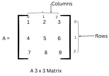
As seen in the image, the elements are organized in rows and columns. These three components are defined as follows:
- Rows: Horizontal arrangement of elements. Matrix A has three rows.
- Columns: Vertical arrangement of elements. Matrix A has three columns.
- Elements: This refers to each data point within the matrix.
The element can be accessed as the intersection of row and column in a matrix. For example, in matrix A, A[0][0] will give the value 1. Note that the matrix elements can be accessed in a manner similar to the elements of a two-dimensional array. In general, an element at the ith row and jth column is accessed as A[i][j].
Key Characteristics of a Matrix
- Dimensions: A matrix is defined by its dimensions, m x n, where m is the number of rows and n is the number of columns.
- Homogeneous Data: All elements within a matrix must be of the same data type (e.g., all integers, all floats).
- Efficient Random Access: Individual elements can be accessed directly using their row and column indices in constant time, O(1). The intersection of a row and a column gives the value of the element.
- Mathematical Operations: Matrices support various mathematical operations like addition, subtraction, multiplication, and transposition, which are fundamental in linear algebra and other fields.
Types of Matrices in Data Structures
There are different types of matrices, each with unique properties and applications in computer science. Some of these are listed here:
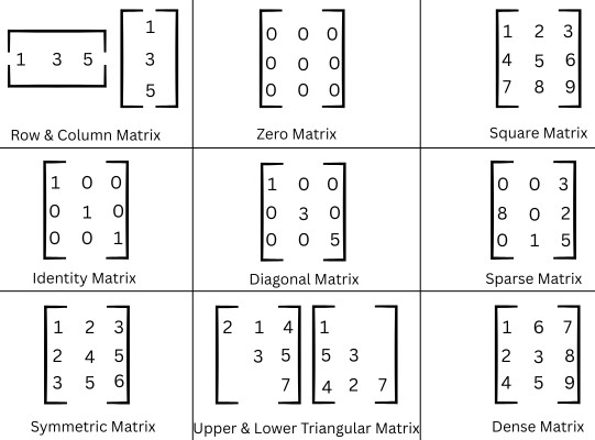
- Row & Column Matrix: A row matrix is a matrix having a single row and n columns. The order of a row matrix is 1 x n. A column matrix, conversely, has m rows and a single column. The order of a column matrix is m x 1.
- Zero Matrix (Null Matrix): A matrix of order m x n is a zero or a null matrix if all elements in the matrix are zero.
- Square Matrix: A matrix with an equal number of rows and columns (m x n where m=n) is a square matrix. A square matrix is used in concepts like determinants, EigenValues, and matrix inversion. A 3 x 3 matrix is a square matrix.
- An identity matrix: This is a square matrix with 1s on the main diagonal and 0s elsewhere.
- Diagonal Matrix: A square matrix where all elements outside the main diagonal are zero. The main diagonal elements are non-zero. Diagonal matrices are optimized for storage, where only diagonal elements (non-zero) are saved.
- Sparse Matrix: A sparse matrix is one where most elements are zero and some are non-zero. A sparse matrix is used extensively in adjacency matrices for graphs, as well as in memory-efficient storage formats such as Compressed Sparse Row (CSR), Compressed Sparse Column (CSC), and Coordinate (COO), where only the non-zero elements are stored. Sparse matrices are also used in recommendation systems and network routing tables.
- Symmetric Matrix: A symmetric matrix is mirrored across the diagonal, such as A[i][j] = A[j][i]. A symmetric matrix is equal to its transpose. It is mainly used in distance matrices and covariance matrices in statistics.
- Upper/Lower Triangular Matrix: The upper and lower triangular matrices are the triangular matrices such that elements above or below the main diagonal are non-zero, respectively. Triangular matrices are used in LU decomposition for solving linear equations.
- Dense Matrix: This is a matrix where most elements are non-zero. A dense matrix is the standard representation and is memory-intensive. It is efficient for compilations where all elements are involved. Dense matrices are used in image-pixel data and transformation matrices in graphics.
Representation of Matrices in Data Structures
Matrices are represented in computer memory in various ways based on their application and efficiency requirements:
1. Row-Major Representation
In this type of representation, matrix elements are stored in contiguous memory locations, one row at a time.
    [ 1  2  3 ]
A=  [ 4  5  6 ]
    [ 7  8  9 ]
1, 2, 3, 4, 5, 6, 7, 8, 9
2. Column-Major Representation
Here, the matrix elements are stored in memory in contiguous locations, one column at a time.
1, 4, 7, 2, 5, 8, 3, 6, 9
3. Sparse Matrix Representation
In this representation, only the non-zero elements of the matrix and their corresponding positions are stored, rather than storing zeros.
- Coordinate List (COO): Stores (row, column, value).
- Compressed Sparse Row (CSR): Stores row pointers and values.
- Compressed Sparse Column (CSC): Similar but column-based.
Sparse matrix representations save memory and speed up operations for large sparse datasets used in social networks and web graphs.
Basic Matrix Operations
Matrices support a variety of operations that are crucial in algorithms:
1. Addition & Subtraction
Addition and subtraction of matrices are possible only if the matrices are of the same order. The addition or subtraction of matrices is carried out element-wise.
For example, if A and B are two matrices, then
A+B = [aᵢⱼ + bᵢⱼ]
The time complexity of this operation is O(n²).
2. Matrix Multiplication
In matrix multiplication, each element is computed as the dot product of the row and the column.
If A is of the order m x n and B is of the order n x p, the resultant matrix C obtained by A x B will have the order m x p.
Basic matrix multiplication has O(n³) complexity, while optimized algorithms, such as Strassen’s, have O(n^2.81) time complexity.
3. Transpose of a Matrix
A matrix is said to be transposed when the rows of a matrix become columns and the columns become rows. Aᵀ denotes the transpose of a matrix.
Hence,
if A = [aᵢⱼ], then Aᵀ = [aⱼᵢ].
The transpose of a matrix is used in machine learning, for example, in gradient descent.
4. Determinants & Eigenvalues
A determinant is a scalar value of a matrix used in matrix inversion and can be calculated for square matrices only. Determinants help solve linear equations and matrix inversion.
Eigenvalues & Eigenvectors are used in PCA (Principal Component Analysis) and stability analysis.
5. Inverse of a Matrix
An inverse of a matrix is a matrix such that A × A⁻¹ = I (Identity matrix). In this case, A⁻¹ is the inverse of a matrix.
The inverse of a matrix is used while tackling problems with conditions and ‘b’ (b equals matrix Ax equation b), this approach is essential, proving invaluable.
6. Traversal & Searching
# Traversing over all the rows
for i in range(0, m-1):
   # Traversing over all the columns of each row
   for j in range(0, n-1):
       print(arr[i][j], end=" ")
   print("")
1 2 3 4
5 6 7 8
9 10 11 12
An element in a matrix can be searched by traversing the matrix.
Applications of Matrices in Computer Science
Matrices are indispensable in computer science and appear in almost every domain. Here are some of the matrix applications in computer science:
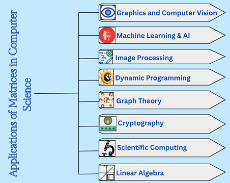
1. Graphics and Computer Vision
Matrices are used in computer vision and graphics to transform images by rotation, scaling, and translation. They can represent 2D and 3D transformations. Matrices are also used for image processing and rendering.
2. Machine Learning & AI
In machine learning & AI, training data is stored as matrices, and they are also used in linear regression and optimization. Matrices represent datasets, implement algorithms such as neural networks, and facilitate statistical analysis. Weight matrices play a central role in neural networks.
3. Image Processing
In image processing, digital images are represented as pixel matrices where each pixel corresponds to an element in a matrix. Convolution matrices are used for filters like blurring and edge detection.
4. Dynamic Programming
Matrices are frequently used in dynamic programming to store the answer to already computed states. Many DP problems, such as edit distance, knapsack, and pathfinding, utilize matrices.
5. Graph Theory
Graphs are represented in computer programming using adjacency matrices. Matrices are also used in shortest path algorithms, such as the Floyd-Warshall algorithm.
6. Cryptography
Encryption and decryption algorithms, such as the Hill Cipher, use matrix transformations in the process.
7. Scientific Computing
Engineering processes, such as finite element analysis (FEA), utilize matrices. Quantum mechanics uses matrices to represent wave functions.
8. Linear Algebra
Matrices are extensively used in linear algebra, a field that deals with linear equations, linear transformations, and vector spaces.
Advantages of Using Matrices in Data Structures
- Multidimensional data can be represented in compact form using matrices.
- Matrix elements can be accessed randomly and are fast, with a time complexity of O(1), as elements can be directly accessed using row and column indices.
- Matrix operations use linear algebra techniques and are very efficient.
- Matrices can handle large datasets and are scalable.
- Matrices can be used for parallel computing.
- They provide support for specialized algorithms in AI, DP, and graphs.
Challenges and Limitations
- Large dense matrices consume vast amounts of memory.
- Operations like matrix multiplication have high time complexity (O(n³) for the naïve approach). However, it is reduced with Strassen or optimized GPU methods.
- Matrices have a fixed size, and resizing them is expensive.
- Sparse matrices’ storage wastes memory. Specialized representations are needed for such matrices.
- Insertion and deletion operations in matrices are costly as they require shifting elements.
Real-World Use Cases of Matrices
- Google Search (PageRank): Google uses matrices for its page ranking algorithm. It utilizes eigenvector computations on the adjacency matrices of the web graph.
- Deep Learning: Tensor operations are generalized using matrices.
- Medical Imaging (MRI, CT scans): Medical imaging techniques, including MRI and CT scans, utilize image matrices analyzed for diagnostic purposes.
- Computer Graphics: 3D games use transformation matrices for rendering objects.
- Weather Prediction: Numerical models rely on matrix computations to predict the weather.
Matrix Data Structure Code Examples
Let us implement the fundamental matrix using C++ and Python programming languages.
Example 1: Matrix Data Structure Representation in C++
#include <iostream>
#include <vector>

class Matrix {
private:
    std::vector<std::vector<int>> data;
    int rows;
    int cols;

public:
    // Constructor
    Matrix(int r, int c) : rows(r), cols(c) {
        data.resize(rows, std::vector<int>(cols, 0)); // Initialize with zeros
    }

    // Access element
    int& operator()(int r, int c) {
        return data[r][c];
    }

    // Const access element
    const int& operator()(int r, int c) const {
        return data[r][c];
    }

    // Print matrix
    void print() const {
        for (int i = 0; i < rows; ++i) {
            for (int j = 0; j < cols; ++j) {
                std::cout << data[i][j] << " ";
            }
            std::cout << std::endl;
        }
    }

    // Getters for dimensions
    int getRows() const { return rows; }
    int getCols() const { return cols; }

    // Matrix addition
    Matrix operator+(const Matrix& other) const {
        if (rows != other.rows || cols != other.cols) {
            throw std::runtime_error("Matrix dimensions must match for addition.");
        }
        Matrix result(rows, cols);
        for (int i = 0; i < rows; ++i) {
            for (int j = 0; j < cols; ++j) {
                result(i, j) = (*this)(i, j) + other(i, j);
            }
        }
        return result;
    }
};

int main() {
    Matrix m1(2, 3);
    m1(0, 0) = 1; m1(0, 1) = 2; m1(0, 2) = 3;
    m1(1, 0) = 4; m1(1, 1) = 5; m1(1, 2) = 6;

    std::cout << "Matrix 1:" << std::endl;
    m1.print();

    Matrix m2(2, 3);
    m2(0, 0) = 7; m2(0, 1) = 8; m2(0, 2) = 9;
    m2(1, 0) = 10; m2(1, 1) = 11; m2(1, 2) = 12;

    std::cout << "\nMatrix 2:" << std::endl;
    m2.print();

    try {
        Matrix sum = m1 + m2;
        std::cout << "\nSum of matrices:" << std::endl;
        sum.print();
    } catch (const std::runtime_error& e) {
        std::cerr << "Error: " << e.what() << std::endl;
    }
   return 0;
}
Matrix 1:
1 2 3
4 5 6

Matrix 2:
7 8 9
10 11 12

Sum of matrices:
8 10 12
14 16 18
Example 2: Matrix Addition and Multiplication in Python
'numpy' library that provides a matrix object with a set of operations.
import numpy as np

# Creating NumPy matrices and printing them
matrix_A = np.array([
    [1, 2, 3],
    [4, 5, 6],
    [7, 8, 9]
])

print ("Matrix A: ")
print(matrix_A)
matrix_B = np.array([
    [9, 8, 7],
    [6, 5, 4],
    [3, 2, 1]
])
print ("Matrix B: ")
print(matrix_B)

# Performing matrix addition)
result_add = matrix_A + matrix_B
print("Matrix Addition:")
print(result_add)

# Performing matrix multiplication
result_mul = np.dot(matrix_A, matrix_B)
print("Matrix Multiplication:")
print(result_mul)
Matrix A:
[[1 2 3]
 [4 5 6]
 [7 8 9]]

Matrix B:
[[9 8 7]
 [6 5 4]
 [3 2 1]]

Matrix Addition:
[[10 10 10]
 [10 10 10]
 [10 10 10]]

Matrix Multiplication:
[[ 30  24  18]
 [ 84  69  54]
 [138 114  90]]
Future of Matrices in Computing
- Tensor Processing Units (TPUs): These are the specialized hardware for matrix operations.
- Quantum Algorithms: Quantum gates used in quantum computing are represented using matrices.
- AI Research: Deep learning relies entirely on efficient tensor/matrix computations.
Conclusion
The matrix data structure is more than just a 2D array. It is, in reality, the backbone of advanced computing, powering critical applications in computer graphics, AI, cryptography, and scientific research.
With a thorough understanding of matrices and their implementation in software programming, developers and data scientists can design efficient algorithms, utilize high-performance computing techniques, and optimize storage. As the realms of AI and quantum computing continue to develop, matrices will remain at the forefront of technological innovation.
|
|