Red-Black Tree in Data Structures: A Complete Guide
When data structures are used in programming, efficient searching, insertion, and deletion operations are crucial for optimizing performance. While simple binary search trees (BST) support these operations with average time complexity of O(logn), their worst-case performance can degrade to O(n) in situations where trees become unbalanced.
This limitation of BST is overcome by self-balancing binary search trees, specifically Red Black Trees and AVL Trees.
The Red Black Tree stands out among these because of its balance between efficiency and flexibility.
| Key Takeaways: |
|---|
|
This article on the Red Black trees provides a complete understanding of Red-Black Trees, including their properties, structures, operations, applications, benefits, and challenges.
What is a Red-Black Tree?
A Red Black Tree (RBT) is a self-balancing BST that maintains additional color information for each node, either red or black, to ensure the balancing of the tree after every modification through insertion and deletion.
RBT uses a color scheme along with a specific set of rules to allow efficient search, insertion, and deletion of nodes with a time complexity of O(logn). Owing to its balancing mechanism, the longest path from the root to any leaf is at most twice as long as the shortest path. This ensures that the time complexity for all tree operations is O(logn).
Properties of Red-Black Trees
- Node Color Property: Every node in an RBT is either red or black.
- Root Property: The root node of an RBT is always black.
- Leaf Property: All leaf nodes (with null children) in RBT are considered black.
- Red Property (No Double Red): No two red nodes in an RBT can be adjacent. In other words, if a node is red, both its children must be black.
- Black-Height Property: In an RBT, every path from a node to its descendant Null nodes must contain the same number of black nodes.
These RBT properties work together in such a way that the tree never becomes unbalanced, thus preserving logarithmic performance.
Real-World Analogy
- Red and Black nodes represent stop and go signals of a traffic system.
- The rules, such as “no two reds together”, ensure a smooth, balanced flow.
- Occasional rotations act like rerouting traffic to avoid congestion.
- This color coding and rotations ensure no “lane” (path) gets too long, keeping operations fast and balanced.
Red Black Tree Visualization: The Structure
A Red Black Tree maintains its balance by using a color coding scheme and rotations. It also follows a specific set of rules to ensure it never gets unbalanced. Before discussing the structure of RBT, let us see the rules that RBT follows.
Red Black Tree Rules
- The root node (top node) is always black.
- Red nodes cannot have red children (no two red nodes can be next to each other).
- Every path from the root to a leaf has the same number of black nodes.
By following these rules, the tree maintains its balance, which helps keep its height (the longest path from the root to a leaf) as short as possible.
Visualization Example
A structure of a Red Black tree consisting of insertions keys { 41, 38, 31, 12, 19, 8, 43,35} is shown below:
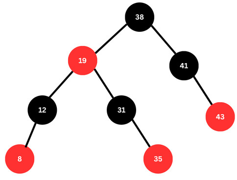
- Root is black.
- No two consecutive nodes are red.
- Equal black height across paths.
How Does the Red Black Tree Maintain the Property of Self-Balancing?
- Recoloring: The colors of the nodes in an RBT are changed to satisfy the Red Black Tree properties after insertions or deletions.
- Rotation: The tree is restructured using left and right rotations to maintain balance and black-height property. The rotations are performed around specific nodes, like parent or grandparent, to re-establish the correct structure.
The color coding scheme that limits the color of the nodes maintains the self-balancing property of the Red Black tree.
RBT Node Structure
struct Node {
  int data;
  Node *parent;
  Node *left;
  Node *right;
  bool color; // RED = true, BLACK = false
};
- Data: The value or key stored in the node.
- Parent, Left, Right: Pointers to parent and left/right child nodes, respectively.
- Color: Indicates whether the node is red or black.
Why Red-Black Tree?
Red Black Trees allow for a less rigid balance while still maintaining logarithmic performance. Due to this reason, RBTs are ideal for use cases where frequent insertions and deletions are required, such as dynamic data structures or real-time systems.
In contrast to RBTs, AVL trees often require more rotations during insertion and deletion.
The following table provides a brief comparison of RBT and AVL Trees:
| Features | Red Black Tree | AVL Tree |
|---|---|---|
| Height Balance | Approximately balanced | Strictly balanced |
| Rotations | Fewer | More frequent |
| Lookup Speed | Slightly slower | Faster |
| Insertion/Deletion | Faster | Slower |
| Use Case | General-purpose, dynamic sets/maps | Static datasets with frequent lookups |
It is seen that though AVL trees are perfectly balanced and faster, they still require more rotations than Red Black trees. This results in slower operations in AVL trees.
- Guaranteed Logarithmic Time Complexity: Red Black trees ensure that all their operations (search, insert, and delete) have a time complexity of O(log n).
- Balanced Structure: The color-coding scheme of Red Black trees ensures that the tree remains relatively balanced, even in worst-case scenarios, preventing slow performance.
- Good Performance in Practice: Red Black trees often have better and faster performance than AVL trees in practice, especially for insertion and deletion operations.
- Widely Used: Red Black trees are used in many standard programming libraries and applications, making them a valuable data structure to understand.
Operations in Red-Black Trees
- Search: Finding elements efficiently within the tree.
- Insertion: Adding new elements (nodes) while maintaining balance in the tree.
- Deletion: Removing elements while preserving Red Black and Binary Search tree properties.
Let us explain each operation in detail.
1. Red-Black Tree Searching
Searching operation in a Red-Black Tree is identical to that in a normal binary search tree.
You traverse left or right based on the comparison of the key to be searched with the current node.
The time complexity for the searching operation is O(log n) (since the height of the tree is logarithmic).
The visual representation of the searching operation is as follows:
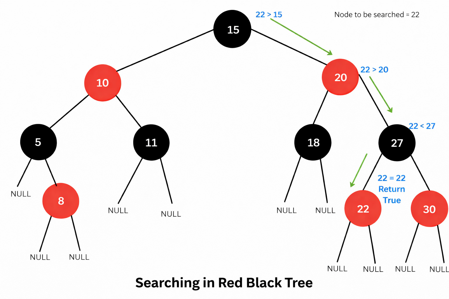
In the above representation, the search path (after comparing the key with nodes) is shown in green. Starting from the root, the search key is repeatedly compared with the nodes in the Red-Black tree to determine the direction of the search. The node values are compared with the search key until the key is found or the last node is traversed.
2. Red-Black Tree Insertion
The insertion operation in a Red Black tree is similar to that in a regular BST, wherein a new node is placed in the correct position. The new node that is inserted is always colored Red.
However, the insertion operation can violate one or more Red-Black tree properties, which must then be corrected using rotations and color flips to ensure balance.
Insertion Cases
- Case 1 – Tree is Empty: The inserted node becomes the root and is colored black.
- Case 2 – Parent is Black: No properties are violated; no adjustments are needed. Node is inserted at its proper position.
- Case 3 – Parent and Uncle are Red: Recoloring parent and uncle to black, and grandparent to red. Then, repeat the balancing process from the grandparent.
- Case 4 – Parent is Red but Uncle is Black: Perform rotation(s) depending on whether the new node is a left or right child, and recolor to restore properties.
Rotations in Red Black Trees
Left Rotation: Promotes the right child and demotes the current node to the left.
x                   y
 \                 /
   y    →    x
 /                 \
  T1                T1
Right Rotation: Promotes the left child and demotes the current node to the right.
       y                x
      /                  \
  x        →            y
      \                  /
       T2               T2
These rotations maintain the BST property while ensuring balance.
Example: Step-by-Step Insertion
The following image shows a sample tree and a node that is inserted in the tree:
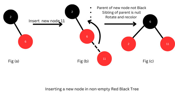
The initial Red Black tree in Fig. (a) consists of two nodes. When the new node with value 11 is inserted, the tree becomes unbalanced as it violates the properties (shown in Fig. (b)).
In this, the parent node of the new node is not black, and the parent sibling is null. Hence, the tree is rotated right and nodes recolored as shown in Fig. (c)
Now, we want to insert another node, 17, in the above Red-Black tree. The insertion process is shown below:
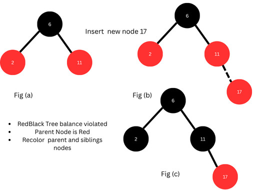
As seen in Fig. (b) above, the balance is violated when a new node is inserted. The parent node (node=11) is red. This balance is restored simply by recoloring the parent and sibling nodes (node 2 and 11 in Fig. c).
3. Red-Black Tree Deletion
Deletion in a Red-Black Tree is more complex than insertion because removing a node may violate multiple properties of the tree. These properties then have to be restored to maintain the balance of the tree.
Steps for Deletion
- If the deleted node or its replacement was red, the tree properties remain intact.
- If a black node is removed, the tree loses one black node on that path, violating the black-height property.
- This imbalance is corrected using a fix-up procedure involving rotations and recoloring.
Deletion Cases
- Case 1 – Sibling is Red: Recolor sibling to black and parent to red, then perform rotation.
- Case 2 – Sibling and its children are black: Recolor sibling to red; move the double-black problem up to the parent.
- Case 3 – Sibling is black, one red child: Perform rotation and recoloring to restore balance.
- Case 4 – Sibling has a red child farther away: Rotate and recolor appropriately.
The time complexity of the deletion operation is O(log n).
Example: Step-by-Step Deletion
Let us perform a deletion operation on a given Red Black tree. Consider the tree shown in the following image:
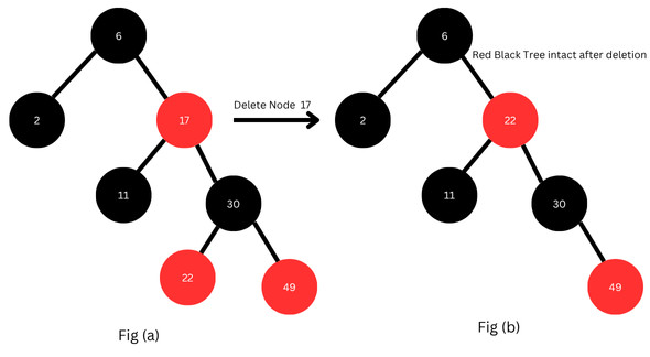
The tree is shown in Fig. (a). We intend to delete node 17 from this tree. This is a red node, and upon deleting it and restructuring, the tree’s balance remains intact.
Next, we want to delete node 22 from the tree. The deletion process is shown below:
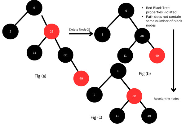
Upon deleting node 22, the tree properties are violated, as all paths do not contain the same number of black nodes (Fig. (b)). To fix this, we recolor the nodes as shown in Fig. (c).
This restores the balance in the Red Black tree.
Red-Black Tree Example Implementation
Red-Black Tree Data Structure in Python
# Node Structure
class Node():
  def __init__(self,val):
    self.val = val
    self.parent = None
    self.left = None
    self.right = None
    self.color = 1

# R-B Tree
class RBTree():
  def __init__(self):
    self.NULL = Node ( 0 )
    self.NULL.color = 0
    self.NULL.left = None
    self.NULL.right = None
    self.root = self.NULL

  # Insert New Node
  def insertNode(self, key):
    node = Node(key)
    node.parent = None
    node.val = key
    node.left = self.NULL
    node.right = self.NULL
    node.color = 1

    y = None
    x = self.root

    while x != self.NULL :
      y = x
      if node.val < x.val :
        x = x.left
      else :
        x = x.right

      node.parent = y
      if y == None :
        self.root = node
      elif node.val < y.val :
        y.left = node
      else :
        y.right = node

      if node.parent == None :
        node.color = 0
        return

      if node.parent.parent == None :
        return

      self.fixInsert ( node )

  def minimum(self, node):
    while node.left != self.NULL:
      node = node.left
    return node

  # left rotate
  def LR ( self , x ) :
    y = x.right
    x.right = y.left

    if y.left != self.NULL :
      y.left.parent = x

    y.parent = x.parent
    if x.parent == None :
      self.root = y
    elif x == x.parent.left :
      x.parent.left = y
    else :
      x.parent.right = y
    y.left = x
    x.parent = y

  # right rotate
  def RR ( self , x ) :
    y = x.left
    x.left = y.right
    if y.right != self.NULL :
      y.right.parent = x

    y.parent = x.parent
    if x.parent == None :
      self.root = y
    elif x == x.parent.right :
      x.parent.right = y
    else :
      x.parent.left = y
    y.right = x
    x.parent = y

  # Fix Up Insertion
  def fixInsert(self, k):
    while k.parent.color == 1:
      if k.parent == k.parent.parent.right:
        u = k.parent.parent.left
        if u.color == 1:
          u.color = 0
          k.parent.color = 0
          k.parent.parent.color = 1
          k = k.parent.parent
        else:
          if k == k.parent.left:
            k = k.parent
            self.RR(k)
          k.parent.color = 0
          k.parent.parent.color = 1
          self.LR(k.parent.parent)
      else:
        u = k.parent.parent.right
        if u.color == 1:
          u.color = 0
          k.parent.color = 0
          k.parent.parent.color = 1
          k = k.parent.parent
        else:
          if k == k.parent.right:
            k = k.parent
            self.LR(k)
          k.parent.color = 0
          k.parent.parent.color = 1
          self.RR(k.parent.parent)
      if k == self.root:
        break
    self.root.color = 0

  # Function to fix issues after deletion
  def fixDelete ( self , x ) :
    while x != self.root and x.color == 0 :
      if x == x.parent.left :
        s = x.parent.right
        if s.color == 1 :
          s.color = 0
          x.parent.color = 1
          self.LR ( x.parent )
          s = x.parent.right
        # If both the children are black
        if s.left.color == 0 and s.right.color == 0 :
          s.color = 1
          x = x.parent
        else :
          if s.right.color == 0 :
            s.left.color = 0
            s.color = 1
            self.RR ( s )
            s = x.parent.right

          s.color = x.parent.color
          x.parent.color = 0
          s.right.color = 0
          self.LR ( x.parent )
          x = self.root
      else :
        s = x.parent.left
        if s.color == 1 :
          s.color = 0
          x.parent.color = 1
          self.RR ( x.parent )
          s = x.parent.left

        if s.right.color == 0 and s.right.color == 0 :
          s.color = 1
          x = x.parent
        else :
          if s.left.color == 0 :
            s.right.color = 0
            s.color = 1
            self.LR ( s )
            s = x.parent.left

          s.color = x.parent.color
          x.parent.color = 0
          s.left.color = 0
          self.RR ( x.parent )
          x = self.root
    x.color = 0

  # Function to transplant nodes
  def __rb_transplant ( self , u , v ) :
    if u.parent == None :
      self.root = v
    elif u == u.parent.left :
      u.parent.left = v
    else :
      u.parent.right = v
    v.parent = u.parent

  # Function to handle deletion
  def delete_node_helper ( self , node , key ) :
    z = self.NULL
    while node != self.NULL :
      if node.val == key :
        z = node

      if node.val <= key :
        node = node.right
      else :
        node = node.left

    if z == self.NULL :
      print ( "Value not present in Tree !!" )
      return

    y = z
    y_original_color = y.color
    if z.left == self.NULL :
      x = z.right
      self.__rb_transplant ( z , z.right )
    elif (z.right == self.NULL) :
      x = z.left
      self.__rb_transplant ( z , z.left )
    else :
      y = self.minimum ( z.right )
      y_original_color = y.color
      x = y.right
      if y.parent == z :
        x.parent = y
      else :
        self.__rb_transplant ( y , y.right )
        y.right = z.right
        y.right.parent = y

      self.__rb_transplant ( z , y )
      y.left = z.left
      y.left.parent = y
      y.color = z.color
    if y_original_color == 0 :
      self.fixDelete ( x )

  # Deletion of node
  def delete_node ( self , val ) :
    self.delete_node_helper ( self.root , val )

  # print Red Black tree
  def __printCall ( self , node , indent , last ) :
    if node != self.NULL :
      print(indent, end=' ')
      if last :
        print ("R---->",end= ' ')
        indent += "     "
      else :
        print("L---->",end=' ')
        indent += "|    "

      s_color = "RED" if node.color == 1 else "BLACK"
      print ( str ( node.val ) + "(" + s_color + ")" )
      self.__printCall ( node.left , indent , False )
      self.__printCall ( node.right , indent , True )

  # Function to call print
  def print_tree ( self ) :
    self.__printCall ( self.root , "" , True )

if __name__ == "__main__":
    rbt = RBTree()

    rbt.insertNode(38)
    rbt.insertNode(19)
    rbt.insertNode(41)
    rbt.insertNode(12)
    rbt.insertNode(31)
    rbt.insertNode(43)
    rbt.insertNode(8)
    rbt.insertNode(35)

    rbt.print_tree()

    print("\nAfter deleting an element")
    rbt.delete_node(43)
    rbt.print_tree()
R----> 38(BLACK)
      L----> 19(RED)
     |     L----> 12(BLACK)
     |    |     L----> 8(RED)
     |     R----> 31(BLACK)
     |           R----> 35(RED)
      R----> 41(BLACK)
           R----> 43(RED)

After deleting an element
 R----> 38(BLACK)
      L----> 19(RED)
     |     L----> 12(BLACK)
     |    |     L----> 8(RED)
     |     R----> 31(BLACK)
     |           R----> 35(RED)
      R----> 41(BLACK)
Complexity Analysis
The following table provides the complexity analysis of the Red Black trees:
| Operation | Best Case | Worst Case | Average Case |
|---|---|---|---|
| Search | O(log n) | O(log n) | O(log n) |
| Insertion | O(1) | O(log n) | O(log n) |
| Deletion | O(log n) | O(log n) | O(log n) |
The logarithmic height of the tree ensures optimal performance.
Applications of Red-Black Trees
- Language Libraries & Data Structures: Common libraries and data structures, such as C++
mapsandsets, as well as Java’sTreeMapandTreeSet, use Red-Black trees for efficient searching and sorting. - Operating Systems: They are used in operating system schedulers to manage processes. For example, Linux utilizes Red-Black trees in process scheduling, virtual memory management, and timer management.
- Databases: Red Black trees are used to implement database indexes, beneficial in efficient searching and retrieval of records.
- Memory Management: Memory allocators utilize Red-Black trees to track free memory blocks efficiently.
- Machine Learning: Red-Black trees are utilized in machine learning algorithms, such as K-means clustering, to reduce time complexity.
- Graph Algorithms: Graph algorithms, such as Dijkstra’s shortest path and Prim’s minimum spanning tree, utilize Red-Black Trees for efficient implementation.
Advantages of Red-Black Trees
- A red-black tree ensures fast operations, such as insertion, deletion, and searching, with an O(log n) time complexity, even in the worst case.
- Compared to AVL Trees, Red-Black Trees require fewer rotations and thus are efficient.
- Red Black trees perform well with continuous insertions and deletions.
- They are ideal for real-world applications where consistent performance matters more than perfect balance.
- Red Black trees automatically balance themselves, ensuring efficient performance without manual intervention.
Disadvantages of Red Black Trees
- Searching in Red Black trees is slightly slower than in AVL trees due to looser balance.
- Red Black trees are complex to implement, as the insertion and deletion balancing rules are challenging to implement.
- Each node in a Red Black Tree requires an additional bit of storage to store its color (red or black), increasing the memory overhead.
- While Red Black Trees offer efficient performance for common operations, they might not always be the optimal choice for every type of data or specific scenarios.
Conclusion
The Red Black tree is one of the most efficient and practical self-balancing tree data structures used in computer science. Operations it provides, like searching, insertion, and deletion, maintain logarithmic complexity by enforcing color-based balance rules.
Its implementation is complex, but its benefits in ensuring consistent performance make it a cornerstone of numerous real-world applications, from programming language libraries to operating systems.
|
|