What is Binary Lifting in DSA?
In the world of Data Structures and Algorithms (DSA), the tree data structure is one of the most fascinating data structures. Many interesting problems are framed in terms of trees. Finding ancestors is one such problem and is addressed by an exquisite and powerful technique called Binary Lifting.
| Key Takeaways: |
|---|
|
This article provides a detailed exploration of binary lifting, covering its intuition, mathematical foundation, algorithmic design, implementation, and practical applications.
Binary Lifting – Working Principle
Binary lifting is a DSA technique used in competitive programming and computer science to efficiently answer queries about ancestors in a tree, such as finding the K-th ancestor or the Lowest Common Ancestor (LCA).
This is achieved by pre-computing the ancestors of each node at powers-of-two distances, allowing for a logarithmic time complexity of O(log N) per query after an initial preprocessing step of O(N log N).

To understand Binary Lifting, let’s first define a common problem in trees:
Given a tree and a node u, find its ancestor at distance k above it (i.e., move k steps up).
A naive approach would involve traversing one parent at a time until we reach the k-th ancestor. This approach, however, takes O(k) time, which is inefficient, especially when k can be as large as N (number of nodes).
- The 1st ancestor of a node is its immediate parent.
- The 2nd ancestor (2¹) is the ancestor of its parent.
- The 4th ancestor (2²) is the ancestor of its 2nd ancestor.
- The 8th ancestor (2³) is the ancestor of its 4th ancestor, and so on.
When these relationships are precomputed for each node, you can jump up the tree in logarithmic time.
- Decompose 13 into powers of two: 13 = 8 + 4 + 1
- Move eight steps up, then four steps up, and then 1 step up. This makes three jumps in total, with a complexity of O (log N) time.
Mathematical Foundation for Binary Lifting
The Binary Lifting technique makes use of the concept of binary representation of numbers and the principles of dynamic programming.
If up[node][i] represents the 2ᶦ-th ancestor of node .
up[node][0]represents the immediate parent of nodeup[node][1]is the 2¹-th ancestor =up[up[node][0]][0]up[node][2]is the 2²-th ancestor =up[up[node][1]][1]- And so on.
The above relationships represent a recursive relation as given here:
up[node][i]=up[up[node][i-1]][i-1]up[node][i] =
up[up[node][i-1]][i-1]up[node][i]=up[up[node][i-1]][i-1]
- To find the 2ᶦ-th ancestor, you can go 2⁽ⁱ⁻¹⁾ steps up twice.
Note: If up[node][i-1] doesn’t exist (e.g., we reached the root), then up[node][i] = -1.
Real-World Analogy
To understand Binary Lifting clearly, let us draw a real-world analogy with an example. Think of Binary Lifting as “teleportation on a ladder.”
If you need to climb 100 rungs, you can either move one step at a time or “teleport” in powers of two, 64 + 32 + 4 (100 rungs), reaching your destination in just a few jumps instead of 100.
Similarly, Binary Lifting allows algorithms to skip intermediate ancestors by precomputing key “teleport points” instead of using a naive approach of traversing one parent at a time to find an ancestor.
How Binary Lifting Works?
The complete process of Binary Lifting is divided into two parts: (1) Preprocessing and (2) Querying the K-th Ancestor. These steps are discussed in detail here:
Preprocessing
The tree needs to be preprocessed before ancestors can be efficiently queried. In these steps, a table up[N][logN] is built where each cell stores the 2ᶦ-th ancestor for each node.
- Build the tree representation using adjacency lists.
- Use DFS from the root to determine:
- The depth of each node.
- The immediate parent of each node.
- Compute up
[node][i]using the recursive relation.
- DFS traversal: O(N)
- Filling the
uptable: O(N log N)
Querying the k-th Ancestor
The next step in binary lifting is querying the k-th ancestor. Once the up table is built in the preprocessing phase, you can find the k-th ancestor of any node using bit decomposition that takes O(log N) time. The algorithm for bit decomposition is given below:
int getKthAncestor(int node, int k) {
    for (int i = 0; i < LOG; i++) {
        if (k & (1 << i)) {     // if i-th bit of k is set
            node = up[node][i];
            if (node == -1) break; // reached root
        }
    }
    return node;
}
- For every bit
iink, check if it’s set. - If yes, move the node to its 2ᶦ-th ancestor.
- Repeat for all bits in
k.
Lowest Common Ancestor (LCA): Binary Lifting Application
Finding the LCS is one of the most common applications of the Binary Lifting technique.
The LCA of two nodes u and v in a tree is the deepest (or lowest) common ancestor of both u and v.
- Distance calculation between nodes.
- Path queries in trees.
- Tree decompositions and network flow algorithms.
LCA Algorithm using Binary Lifting
-
Step 1: Equalize Depths
From the above definition of LCA, ifuandvare at different depths, lift the deeper node until both are at the same level. -
Step 2: Lift Both Nodes Together
Starting from the highest power of two down to zero, ifup[u][i] != up[v][i], lift bothuandvby 2ᶦ. -
Step 3: Final Step
Whenuandvhave the same parent, that parent is their LCA.
The following code provides the implementation of LCA:
int LCA(int u, int v) {
    if (depth[u] < depth[v])
        swap(u, v);
    // Step 1: Equalize depths
    int diff = depth[u] - depth[v];
    u = getKthAncestor(u, diff);
    if (u == v) return u;
    // Step 2: Lift both up
    for (int i = LOG - 1; i >= 0; i--) {
        if (up[u][i] != up[v][i]) {
            u = up[u][i];
            v = up[v][i];
        }
    }
    // Step 3: Parent is LCA
    return up[u][0];
}
- Preprocessing: O(N log N)
- Query: O(log N)
- Space: O(N log N)
Example Walkthrough for Binary Lifting and LCA
Let’s consider a simple example with the following tree:
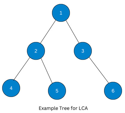
Now we will walk through the Binary Lifting technique to find the LCA of nodes.
Step 1: Build up a table for up[node][0] (immediate parent)
The following is the table up[node][0] that shows each node with its immediate parent as seen from the tree above:
1 ->-1 |
|---|
2 ->1 |
3 ->1 |
4 ->2 |
5 ->2 |
6 ->3 |
Next, build table up[node][1] (2 ancestors above)
This table contains the list of nodes with two ancestors above:
2 ->-1 |
|---|
3 ->-1 |
4 ->1 |
5 ->1 |
6 ->1 |
Step 2: Find LCA
Case 1
Let us assume that we need to find the LCA for nodes 4 and 5, LCA(4, 5). The finding of LCA is depicted in the image below:
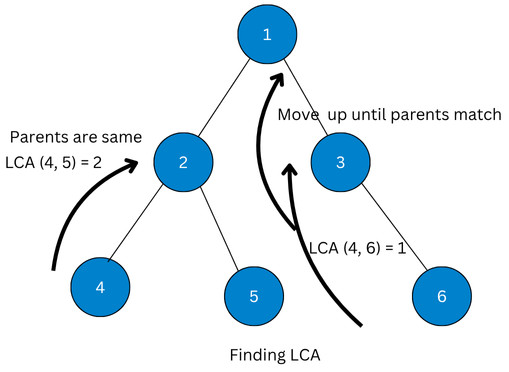
- Check the depth of the nodes 4 and 5. From the diagram, we can see that both nodes are at depth 2.
- According to the algorithm, since the depths of the two nodes are the same, and from the
uptable above,
up[4][0] = 2, up[5][0] = 2
Hence, LCA (4,5) = 2.
Case 2
- The first step is to equalize the depths of nodes. In this case, both nodes are at level 2.
- The next step is to check the parents. In this case, the parents of both nodes are different. Therefore, we move both up until parents match by referring to the
uptable.
up[4][1] = 1, up[6][1] = 1
Now that both parents are matching, the LCA(4,6) = 1.
Applications of Binary Lifting
The Binary Lifting technique has become important in modern algorithmic design. Here are some applications of the Binary Lifting technique:
1. Tree Queries
- Distance between nodes.
- Finding k-th ancestors.
- Path sum or maximum edge weight queries (with modifications).
2. Heavy-Light Decomposition
The Binary Lifting technique is used as a subcomponent in segment tree structures for advanced tree queries.
3. Range Queries in Graphs
The Binary Lifting technique extends beyond trees to Directed Acyclic Graphs (DAGs) for establishing ancestor relationships.
4. Game Trees and AI
In turn-based or hierarchical decision-making systems, the Binary Lifting technique facilitates the efficient simulation of “jumping” multiple levels in logarithmic time.
5. Dynamic Programming on Trees
The Binary Lifting technique is used in DP problems where subproblem dependencies involve ancestors.
Space and Time Complexity Analysis
The following table shows the time complexities for individual operations in the Binary Lifting and the LCA algorithm:
| Operation | Complexity |
|---|---|
| Preprocessing | O(N log N) |
| LCA Query | O(log N) |
| K-th Ancestor Query | O(log N) |
| Space | O(N log N) |
Though Binary Lifting’s preprocessing seems heavy, it’s well worth it for applications involving multiple queries, such as competitive programming problems or large-scale computations on static trees.
Advantages and Limitations of Binary Lifting
Advantages
- The Binary Lifting technique is highly efficient for multiple ancestors or LCA queries.
- It is simple to implement compared to other LCA algorithms (like Tarjan’s offline method).
- This technique works well on static trees (no modifications between queries).
- After preprocessing, queries like finding the k-th ancestor or LCA can be answered in O(log N) time.
- The Binary Lifting technique is significantly faster for repeated queries than repeatedly traversing the tree from scratch.
- The precomputed ancestor information can be used to solve other tree problems, such as finding path sums or minimums.
Limitations
- The Binary Lifting technique has high memory usage with O(N log N) space complexity. This may be impractical for huge trees.
- Its static structure is not suitable for dynamic trees where nodes are added or removed.
- When queries are few, the preprocessing phase might not be worth the cost.
Common Variations of the Binary Lifting Technique
- Weighted Binary Lifting: This technique stores additional data (e.g., max/min edge weights) along with ancestors. Weighted Binary Lifting is used in path queries and network design.
- Binary Lifting for DAGs: The Binary Lifting technique can be adapted for graphs without cycles in addition to trees.
- Dynamic Binary Lifting: This is an advanced variant of the Binary Lifting technique that allows updates with segment trees or link-cut trees.
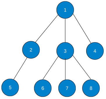
Practical Example of Binary Listing & LCA
Below is a working C++ implementation for Binary Lifting and LCA. For this program, the input is the following tree:
#include <bits/stdc++.h>
using namespace std;

// Pre-processing phase
void dfs(int u, int p, int **upTab, vector<int> &node_level, int log, vector<int> *g)
{
    // update upTab
    upTab[u][0] = p;
    for (int i = 1; i <= log; i++)
        upTab[u][i] = upTab[upTab[u][i - 1]][i - 1];
    for (int v : g[u])
    {
        if (v != p)
        {
            node_level[v] = node_level[u] + 1;
            dfs(v, u, upTab, node_level, log, g);
        }
    }
}

// returns LCA (u, v)
int lca(int u, int v, int log, vector<int> &node_level, int **upTab)
{
    if (node_level[u] < node_level[v])
        swap(u, v);

    // Find the ancestor of u at the same level as v
    for (int i = log; i >= 0; i--)
        if ((node_level[u] - pow(2, i)) >= node_level[v])
            u = upTab[u][i];

    // If v is the ancestor of u, then v is the LCA of u and v
    if (u == v)
        return u;

    for (int i = log; i >= 0; i--)
    {
        if (upTab[u][i] != upTab[v][i])
        {
            u = upTab[u][i];
            v = upTab[v][i];
        }
    }
    return upTab[u][0];
}

int main()
{
    // Max Number of nodes
    int n = 10;

    vector<int> treeList[n + 1];     // vector to store tree

    int log = (int)ceil(log2(n));
    int **upTab = new int *[n + 1];
    for (int i = 0; i < n + 1; i++)
        upTab[i] = new int[log + 1];

    vector<int> node_level(n + 1);   // Stores the level of each node

    for (int i = 0; i <= n; i++) //Initialize upTab values to -1
       memset(upTab[i], -1, sizeof upTab[i]);

    // Add edges to the tree
    treeList[1].push_back(2);
    treeList[2].push_back(1);
    treeList[1].push_back(3);
    treeList[3].push_back(1);
    treeList[1].push_back(4);
    treeList[4].push_back(1);
    treeList[2].push_back(5);
    treeList[5].push_back(2);
    treeList[3].push_back(6);
    treeList[6].push_back(3);
    treeList[3].push_back(7);
    treeList[7].push_back(3);
    treeList[3].push_back(8);
    treeList[8].push_back(3);

    dfs(1, 1, upTab, node_level, log, treeList);
    cout << "LCA(5, 6) = " << lca(5, 6, log, node_level, upTab) << endl;
    cout << "LCA(5, 1) = " << lca(5, 1, log, node_level, upTab) << endl;
    cout << "LCA(6, 4) = " << lca(6, 4, log, node_level, upTab) << endl;
    cout << "LCA(6, 8) = " << lca(6, 8, log, node_level, upTab) << endl;

    return 0;
}
The output of this program is given below:
LCA(5, 6) = 1
LCA(5, 1) = 1
LCA(6, 4) = 1
LCA(6, 8) = 3
Conclusion
Binary Lifting is one of those highly efficient algorithmic techniques that combine mathematical elegance with practical efficiency. With this technique, the tree traversal is transformed from a linear-time problem into a logarithmic-time solution using a simple dynamic programming principle.
Whether it is preparing for coding interviews, competitive programming, or building optimized graph algorithms, mastering Binary Lifting will empower developers to solve complex tree problems with speed and clarity.
Additional Resources
- Why Learning Data Structures and Algorithms (DSA) is Essential for Developers
- What is Code Optimization?
- Searching vs Sorting Algorithms: Key Differences, Types & Applications in DSA
|
|