What is Recursion in Data Structures
Recursion is regarded as one of the most fundamental and fascinating concepts in computer science and data structures. From searching and sorting to parsing and mathematical computations, recursion forms the backbone of many algorithms. Recursion is defined as a technique in which a function calls itself directly or indirectly to reach a specific solution.
| Key Takeaways |
|---|
|
In this article, we will explore the concept of recursion, discuss its importance, types, and applications. We will also examine the recursion from a programming perspective.
Recursion in Data Structures
In computer programming, recursion is a process in which a function calls itself during its execution until a specific condition known as the base case is met.

For example, consider the mathematical factorial function defined as:
N! = N * (N-1) * (N-2) *...1
If you want to calculate the factorial of the number 5, it is given by
5! = 5 * 4 * 3 * 2 * 1 = 120
If you want to program the function to calculate the factorial of a number N, from the above example, you can deduce that we will end up with the same calculation until we reach N = 1. This will unnecessarily increase the length of the code, especially when N has higher values.
Instead, we use a function that basically implements the general procedure of calculating the factorial, but we call this function every time with a different argument. This is where recursion comes into the picture.
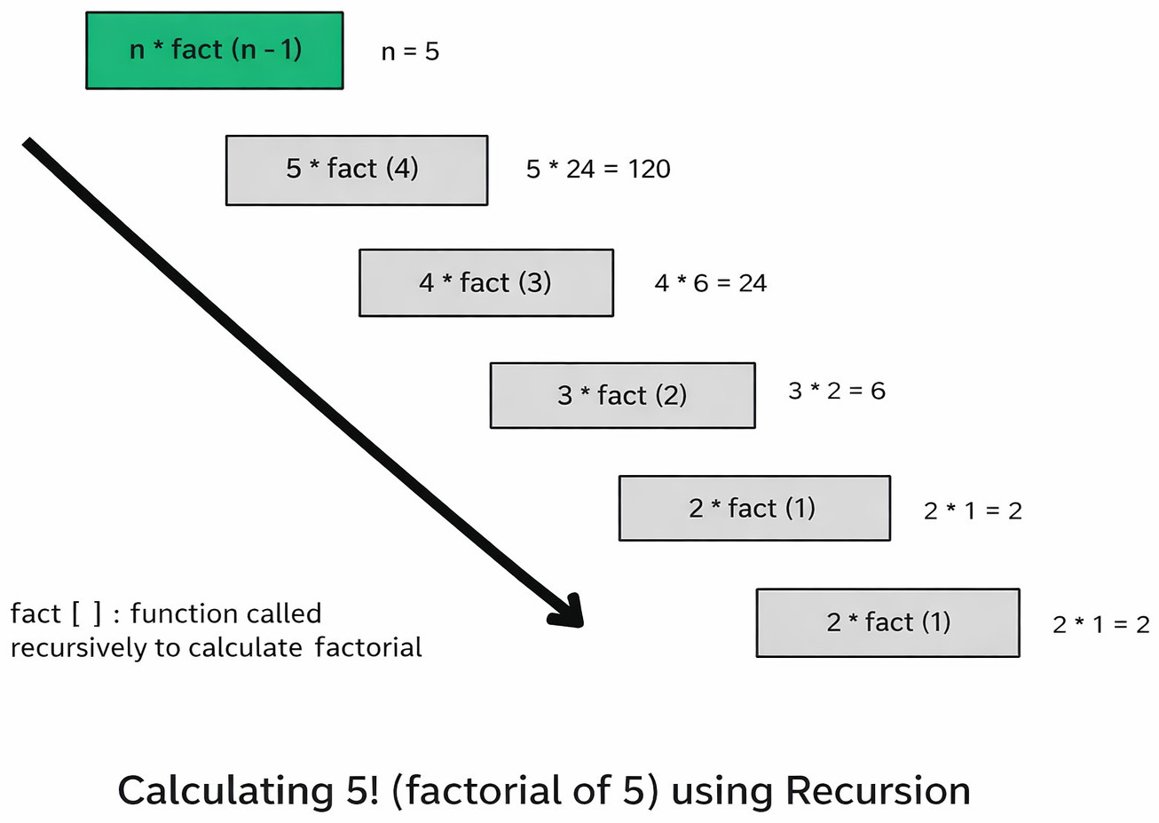
def factorial(n):
  if n == 0:
    return 1
  else:
    return n * factorial(n - 1)   # recursive call
The pictorial representation of the above code is shown as:
- The function
factorial()calls itself with a smaller argument (n-1). - The base case is
n == 0, which means when n reaches 0, the function will exit. - The recursive case progressively reduces the problem size after every iteration.
When a recursive function is called, each invocation is pushed onto the call stack, which stores information about active subroutines.
For example, in the above factorial example (factorial(4)):
factorial(4) calls factorial(3), factorial(3) calls factorial(2), and so on till factorial(0) returns 1. After that, each pending call returns in reverse order.
This last-in-first-out (LIFO) behavior is precisely how the call stack in recursion operates.
Base Case and Recursive Case
- Base Case: The condition under which recursion terminates. In the above pseudo code, if you remove the condition
'if n == 0', the program will continue to run the recursive call indefinitely. In this case, the program stack will be exhausted, causing a Stack Overflow error. - Recursive Case: This is the part of the function where it calls itself with a modified parameter. In the above pseudo code, it is the call to the
factorialfunction with a different value of N.
Steps to Implement Recursion
- Define a Base Case: Identify the simplest (or base) case for the solution. This is the case for which the solution is trivial. This acts as the terminating condition for the recursion.
- Define a Recursive Case: Break down the problem into smaller subproblems and express each as a smaller version of itself. This way, the function can be called recursively to solve each subproblem.
- Ensure the Recursion Terminates: Ensure that the recursive call ultimately meets the base condition and terminates successfully after all subproblems are solved.
- Combine the Solutions: Combine the solutions of the subproblems to solve the original problem.
Types of Recursion in Data Structures
Recursion is classified into various types as follows:
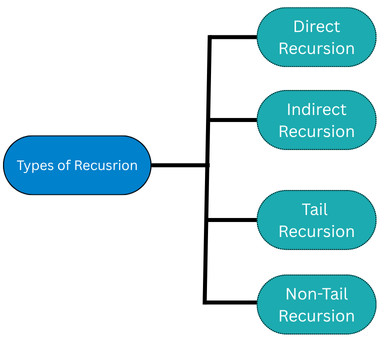
Direct Recursion
- Direct recursion simplifies mathematical computations, such as those involving factorials or Fibonacci sequences.
- It is the backbone of many dynamic programming solutions.
- Direct recursion is commonly used in traversing trees or graphs.
- Direct recursion needs a well-defined base case for its termination.
- It is easier to debug and visualize as it has a linear nature.
#include <iostream>
using namespace std;

int fact(int n)
{
  if (n == 0)         // BASE case
    return 1;

  return n * fact(n - 1);
}

int main()
{
  cout << "Factorial of 20: " << fact(10);
  return 0;
}

OUTPUT:
Factorial of 20: 3628800
Indirect Recursion
Indirect recursion occurs when a function calls another function, which in turn calls the original function, thereby generating a cycle between two or more tasks that leads to recursion.
- Multi-step problems involving two or more functions.
- Mutual recursion where interdependent tasks work together.
- Compiler design and expression evaluations.
- Adds complexity to code.
- Requires careful tracking of function calls to maintain clarity.
even and odd, call each other recursively using indirect recursion.
#include <iostream>
using namespace std;
int odd (int n);
int even(int n){
  if (n == 0)
    return 1;
  else
    return odd(n - 1);
}

 int odd(int n){
  if (n == 0)
    return 0;
  else
    return even(n - 1);
}
int main()
{
  int retval = even (1);
  if (retval == 1)
    cout << "The number is even";
  else
    cout << "The number is odd";

  return 0;
}

Output:
The number is odd
Tail Recursion
Tail recursion occurs when the recursive call is the last operation in the function. At this point, the function returns the result of the recursive call directly, without performing any further operations after executing it.
Tail-recursive functions allow optimizations like Tail Call Optimization (TCO), wherein the compiler can reuse the current function’s stack frame, thus saving memory and making recursion more efficient.
- It reduces memory overhead by allowing compilers to optimize the recursive call.
- Tail recursion is standard in situations where intermediate results aren’t needed.
- It simplifies mathematical series or iterative tasks.
- Tail recursion enables recursion to duplicate an iterative loop.
- It is ideal for problems requiring large recursion depths.
#include <iostream>
using namespace std;

int fact(int n, int result=1)
{
  if (n == 1)         // BASE case
    return result;

  return fact(n - 1, n * result);   //tail recursion
}

int main()
{
  cout << "5! : " << fact(5);
  return 0;
}

Output:
5! : 120
Non-Tail Recursion
In non-tail recursion, the recursive function is not the last operation in the function. After the recursive call returns the value, additional statements/functions are performed. Hence, each stack frame must be maintained for each recursive call, resulting in higher memory usage and a potential stack overflow for deep recursions.
- Non-tail recursion retains intermediate computations for tasks like tree traversals.
- It allows flexibility in solving layered problems.
- Memory usage increases in non-tail-recursive functions due to the additional stack frames required.
- It is commonly used in algorithms like DFS or complex mathematical computations.
- Non-tail recursion requires precise control to avoid excessive stack overhead.
Any function that does not have recursion as the last statement is an example of non-tail recursion. The factorial program demonstrated in direct recursion is also an example of non-tail recursion.
Applications of Recursion in Data Structures
Recursion is very important in various data structure algorithms. Some key applications include:
Recursion with Linked Lists
A linked list, which is a collection of nodes, is inherently recursive because each node contains data and a reference pointer to the next node, which is itself a linked list. Various linked list operations, such as traversing a linked list, reversing a linked list, or searching for an element in the linked list, can be performed using recursion.
def print_list(node):
  if node is None:
      return
  print(node.data)
  print_list(node.next)
Here, the linked list is traversed from the start, and for each node, its data is printed. The same function is then called again with the next pointer of the current node as an argument.
Recursion simplifies operations like traversal, insertion, and deletion in linked lists.
Recursion in Trees
A tree data structure consisting of a root node and subtrees is defined recursively, and they are where the recursion shines:
- Inorder Traversal (Left → Root → Right)
The steps for inorder tree traversal are:
- Start at the root node.
- Recursively visit the left subtree.
- Visit the root node.
- Recursively visit the right subtree.
The pseudo-code for the same is as follows:Inorder(node): if node is not null: Inorder(node.left) Visit(node) Inorder(node.right) - Preorder Traversal (Root → Left → Right)
Step-by-step preorder traversal is:
- Start at the root node.
- Visit the root node.
- Recursively visit the left subtree.
- Recursively visit the right subtree.
Here is the pseudo-code for preorder traversal:Preorder(node): if node is not null: Visit(node) Preorder(node.left) Preorder(node.right) - Postorder Traversal (Left → Right → Root)
Postorder traversal is performed using the following steps:
- Start at the root node.
- Recursively visit the left subtree.
- Recursively visit the right subtree.
- Visit the root node.
The pseudo-code for postorder traversal:Postorder(node): if node is not null: Postorder(node.left) Postorder(node.right) Visit(node)
Although the system’s call stack is used internally for recursion, the tree data structure does not utilize any explicit data structure, such as a stack or a queue, when traversing the tree recursively.
Recursion in Graphs
Graph algorithms use traversal techniques to explore all nodes or search for specific elements. Depth-First Search (DFS) uses recursion to explore deeper into the graph, while Breadth-First Search (BFS) iterates through the graph level by level.
- Start at the root or any node.
- Mark the current node as visited.
- Recursively visit each unvisited neighbor of the current node.
- Backtrack if all neighbors have been visited.
def dfs(graph, node, visited):
  if node not in visited:
    print(node)
    visited.add(node)
    for neighbor in graph[node]:
      dfs(graph, neighbor, visited)
This recursive DFS explores all nodes connected to the starting node by following paths recursively until no unvisited nodes remain.
Searching and Sorting Algorithms
Recursion is extensively used in searching and sorting algorithms. Searching algorithms like binary search recursively divide the array to find an element. Sorting algorithms divide the problem into smaller subproblems, which are recursively sorted and combined to achieve a fully sorted list. Merge sort and quicksort are two algorithms that utilize recursion.
- Binary Search: Recursively divides the array to find an element.
The pseudo code for binary search using recursion is as follows:
def binary_search(arr, low, high, key): if low > high: return -1 mid = (low + high) // 2 if arr[mid] == key: return mid elif arr[mid] > key: return binary_search(arr, low, mid - 1, key) else: return binary_search(arr, mid + 1, high, key) - Merge Sort: divides the array into halves, sorts recursively, and merges the two arrays. This process is continued till the entire array is sorted.
The pseudo-code for merge sort is:
MergeSort(arr): if len(arr) > 1: mid = len(arr) // 2 left_half = arr[:mid] right_half = arr[mid:] MergeSort(left_half) MergeSort(right_half) Merge(arr, left_half, right_half) Merge(arr, left_half, right_half): i = j = k = 0 while i < len(left_half) and j < len(right_half): if left_half[i] < right_half[j]: arr[k] = left_half[i] i += 1 else: arr[k] = right_half[j] j += 1 k += 1 while i < len(left_half): arr[k] = left_half[i] i += 1 k += 1 while j < len(right_half): arr[k] = right_half[j] j += 1 k += 1 - Quick Sort: This algorithm partitions the array around a pivot and sorts subarrays recursively.
The pseudo-code for the quick sort algorithm using recursion is as follows:
QuickSort(arr, low, high):
  if low < high:
    pivot = Partition(arr, low, high)
    QuickSort(arr, low, pivot - 1)
    QuickSort(arr, pivot + 1, high)

Partition(arr, low, high):
  pivot = arr[high]
  i = low - 1
  for j = low to high - 1:
    if arr[j] < pivot:
      i = i + 1
      Swap(arr[i], arr[j])
  Swap(arr[i + 1], arr[high])
  return i + 1
Dynamic Programming
Many dynamic programming problems, such as the Fibonacci series, knapsack problem, and matrix chain multiplication, start with a recursive definition and are optimized using memoization.
The Fibonacci series is denoted as 0, 1, 1, 2, 3, 5, 8, 13, …
The next number in a Fibonacci series is the sum of the previous two numbers. Hence, the nth term in the Fibonacci series is given by,
F(n) = F(n-1) + F(n-2)
def fib(n):
  if n <= 1:
    return n
  return fib(n-1) + fib(n-2)
Backtracking
Backtracking problems such as the N-Queens Problem, Sudoku Solver, and Maze Pathfinding use recursion extensively. Each recursive call explores a possible path and backtracks when the constraints are not met.
Real-World Examples of Recursion in Data Structures
- File System Navigation: Recursion is used for effortless navigation of directories. It explores nested directories, mimicking the structure of a tree. Using recursion, the files are processed layer by layer, making organization manageable.
- Compilers and Parsers: Recursion is used in low-level programming of compilers and parsers, like recursive descent parsing of expressions.
- Computer Graphics: Recursion is helpful in computer graphics for generating fractals, subdivision surfaces, or recursive patterns. The approach helps graphic rendering in computer graphics and nature simulations.
- Web Crawling: Crawlers use recursion to traverse web pages. They fetch links from a page, follow each one recursively, and build comprehensive datasets.
- AI and Puzzles: Many puzzles in AI, like Sudoku, the N-Queens problem, and game strategies in AI use recursive backtracking, wherein every possible move is evaluated to identify the winning solution.
- Tree Traversal: Recursion is key in traversing tree-like data structures, such as binary trees, and performing operations like search, insert, or delete nodes.
Advantages and Disadvantages of Recursion
The following table summarizes the advantages and disadvantages of recursion:
| Advantages of Recursion | Disadvantages of Recursion |
|---|---|
| Simplicity: Recursive algorithms are often simple, more readable, and closer to mathematical formulations. | Memory Overhead: Each recursive call consumes stack space and more memory. |
| Reduction in Code Size: Recursion means fewer lines of code. | Performance Issues: Too much recursion may result in exponential time complexity. |
| Natural Fit for Recursive Data Structures: Recursion works seamlessly with trees and graphs. | Stack Overflow: Deep recursion may exceed the system’s call stack limit. |
| Elegant Implementation: Recursion is useful in traversal, searching, and hierarchical data processing. | Difficult Debugging: Tracing and debugging recursive calls can be harder compared to iterative methods. |
Recursion vs Iteration
Recursion and iteration are used to execute repetitive code. However, they differ in how they execute and store intermediate results. Here are the key differences between recursion and iteration:
| Aspect | Recursion | Iteration |
|---|---|---|
| Mechanism | A recursive function calls itself repeatedly until a base condition is satisfied | Iteration loops through a code using looping constructs (for, while) |
| Termination | Base case | Loop condition |
| Memory Usage | Uses the call stack to save the intermediate state | Uses loop variables |
| Performance | Can be slower | Usually faster |
| Readability | More expressive, elegant | More explicit and procedural |
| Code Size | Smaller | Larger |
When to Use Recursion?
- When the problem can be broken into smaller subproblems of the exact nature.
- If there exists a well-defined base case.
- When the recursive solution is more intuitive than the iterative one.
- If the stack memory consumption is within limits.
- Iterative solutions are simpler and more efficient compared to recursion.
- The problem involves deep recursion, resulting in a stack overflow.
- Performance optimization is critical.
Conclusion
Recursion is an essential concept in computer science and data structures. It elegantly expresses repetitive or hierarchical problems. It is deeply connected with data structures like trees, graphs, and linked lists, as these data structures are designed recursively.
Recursion represents not only a programming language feature but also a way of thinking about problems, breaking them down into smaller subproblems until the solution naturally emerges.
Recursion, however, must be used responsibly and judiciously to avoid inefficiencies and stack overflows. Understanding the working of recursion, its advantages and disadvantages, and its relationship with data structures enables professionals to develop cleaner, powerful, and maintainable applications.
|
|